Visualising Underfitting and Overfitting in High Dimensional Data
Visualising Underfitting and Overfitting in High Dimensional Data
Welcome! This workshop is from Winder.ai. Sign up to receive more free workshops, training and videos.
In the previous workshop we plotted the decision boundary for under and overfitting classifiers. This is great, but very often it is impossible to visualise the data, usually because there are too many dimensions in the dataset.
In thise case we need to visualise performance in another way. One way to do this is to produce a validation curve. This is a brute force approach that repeatedly scores the performanc of a model on holdout data for each parameter that you specify.
But the coolest thing about sklearns implementation is that it performs cross-validation. This means the approach is quite reliable and we get some statistical confidence about our scores.
In short, we perform a grid search over various values of hyperparameters to control the fitting of the model.
# Usual imports
import os
import pandas as pd
import matplotlib.pyplot as plt
import numpy as np
from IPython.display import display
from sklearn.model_selection import train_test_split
from sklearn.datasets import make_circles
from sklearn.svm import SVC
# Synthetic data
X, y = make_circles(noise=0.2, factor=0.5, random_state=1, n_samples=200)
# Use sklearns inbuilt validation_curve method
# Although it wouldn't be too hard to code ourselves.
from sklearn.model_selection import validation_curve

param_range = np.logspace(-2, 3, 10)
train_scores, test_scores = validation_curve(
    SVC(), X, y, param_name="gamma", param_range=param_range,
    cv=10, scoring="accuracy", n_jobs=1)

# Generate average scores and standard deviations for more interesting plots
train_scores_mean = np.mean(train_scores, axis=1)
train_scores_std = np.std(train_scores, axis=1)
test_scores_mean = np.mean(test_scores, axis=1)
test_scores_std = np.std(test_scores, axis=1)
# Plot the results
plt.figure()
lw = 2
plt.semilogx(param_range, train_scores_mean, label="Training score",
             color="darkorange", lw=lw)
plt.fill_between(param_range, train_scores_mean - train_scores_std,
                 train_scores_mean + train_scores_std, alpha=0.2,
                 color="darkorange", lw=lw)
plt.semilogx(param_range, test_scores_mean, label="Cross-validation score",
             color="navy", lw=lw)
plt.fill_between(param_range, test_scores_mean - test_scores_std,
                 test_scores_mean + test_scores_std, alpha=0.2,
                 color="navy", lw=lw)

plt.title("Validation Curve (SVM)")
plt.xlabel("$\gamma$")
plt.ylabel("Score")
plt.ylim(0.01, 1.1)
plt.grid()
plt.legend(loc="best")
plt.show()
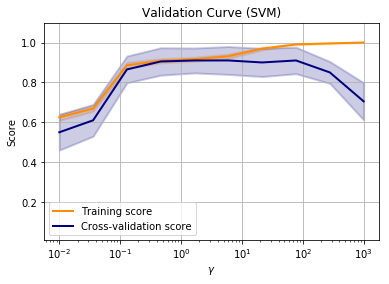
Now it is clear that the best value for gamma is somewhere around a value of 1-10. The beauty is that this works on data of any number of dimensions.
But it does get tricky when you have multiple parameters to tune. For this we have to perform a grid search. A grid search is a repeated training and fitting proces over many different hyperparameters.
Learning curves
Another way of visualising performance is with a learning curve. This plot uses different size samples to perform the training.
If there is a large gap between the train and validation score, then we are overfitting. If the training score is low, we are underfitting.
If we can see the learning curve continue to rise with more samples, then we might get better performance if we collected more samples.
# Use sklearns inbuilt validation_curve method
# Although it wouldn't be too hard to code ourselves.
from sklearn.model_selection import learning_curve
param_range = np.logspace(-1.3, -0.1, 10)
train_sizes, train_scores, test_scores = learning_curve(
    SVC(), X, y,
    train_sizes=param_range, cv=5)

# Generate average scores and standard deviations for more interesting plots
train_scores_mean = np.mean(train_scores, axis=1)
train_scores_std = np.std(train_scores, axis=1)
test_scores_mean = np.mean(test_scores, axis=1)
test_scores_std = np.std(test_scores, axis=1)
# Plot the results
plt.figure()
lw = 2
plt.semilogx(param_range, train_scores_mean, label="Training score",
             color="darkorange", lw=lw)
plt.fill_between(param_range, train_scores_mean - train_scores_std,
                 train_scores_mean + train_scores_std, alpha=0.2,
                 color="darkorange", lw=lw)
plt.semilogx(param_range, test_scores_mean, label="Cross-validation score",
             color="navy", lw=lw)
plt.fill_between(param_range, test_scores_mean - test_scores_std,
                 test_scores_mean + test_scores_std, alpha=0.2,
                 color="navy", lw=lw)

plt.title("Validation Curve (SVM)")
plt.xlabel("$\gamma$")
plt.ylabel("Score")
plt.ylim(0.01, 1.1)
plt.grid()
plt.legend(loc="best")
plt.show()
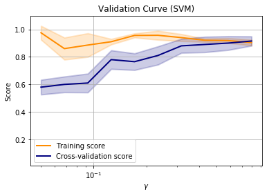
Note that in this example, the training score and cross-validation score are approximately equal when all of the training data is used.
This is suggesting that adding more data will not improve performance and we are performing as well as we can with this model. At this point we might want to consider other models to improve the training score.
from sklearn.datasets import make_moons

# Synthetic data
X, y = make_moons(noise=0.2, random_state=42)

# This is how we split our data, using the `train_test_split` method
X_train, X_test, y_train, y_test = \
    train_test_split(X, y, test_size=.4, random_state=42)
Tasks
- Fit a Support Vector Machine to the above “moons” data.