Testing Model Robustness with Jitter

Welcome! This workshop is from Winder.ai. Sign up to receive more free workshops, training and videos.

To test whether your models are robust to changes, one simple test is to add some noise to the test data. When we alter the magnitude of the noise, we can infer how well the model will perform with new data and different sources of noise.

In this example we’re going to add some random, normally-distributed noise, but it doesn’t have to be normally distributed! Maybe you could add some bias, or add some other type of trend!

from sklearn import metrics, datasets, naive_bayes, svm, tree
import numpy as np
from matplotlib import pyplot as plt
from sklearn.model_selection import train_test_split
from pandas import Series
from matplotlib import pyplot

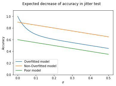
What we would expect is something like the following. If we have a model that grossly overfits the data, it is likely to start high (e.g. lookup table). Because it hasn’t made any generalisations, as soon as we start adding noise performance will quickly drop.

x = np.linspace(0, 0.5, 100)

plt.plot( x, 0.7 - 0.5*x + 0.3*np.exp(-x*20), label = "Overfitted model")
plt.plot( x, 0.9 - 0.5*x, label = "Non-Overfitted model")
plt.plot( x, 0.6 - 0.5*x, label = "Poor model")

axes = plt.gca()
axes.set_ylim([0, 1.1])

plt.legend(loc=3)
plt.suptitle("Expected decrease of accuracy in jitter test")

axes.set_xlabel('$\sigma$')
axes.set_ylabel('Accuracy')

plt.show()

Jitter methods

“Jitter” is simply some noise added to the original signal.

Below a jitter_test runs a prediction on the new jitter data over several different jitter scales (standard deviations). To make the resulting curves a little smoother, we’re performing the experiment several times and taking the average.

def jitter(X, scale=0.1):
    return X + np.random.normal(0, scale, X.shape)

def jitter_test(classifier, X, y, scales = np.linspace(0, 0.5, 30), N = 5):
    out = []
    for s in scales:
        avg = 0.0
        for r in range(N):
            avg += metrics.accuracy_score(y, classifier.predict(jitter(X, s)))
        out.append(avg / N)
    return out, scales

Below we’re generating the test data. We’re using the moons dataset to make it quite difficult.

np.random.seed(1234)
X, y = datasets.make_moons(n_samples=200, noise=.3)

mdl1 = svm.SVC()
mdl1.fit(X, y)

mdl2 = tree.DecisionTreeClassifier()
mdl2.fit(X,y);

mdl1_scores, jitters = jitter_test(mdl1, X, y)
mdl2_scores, jitters = jitter_test(mdl2, X, y)

plt.figure()
lw = 2
plt.plot(jitters, mdl1_scores, color='darkorange',
         lw=lw, label='SVM')
plt.plot(jitters, mdl2_scores, color='blue',
         lw=lw, label='Decision Tree')
plt.xlabel('Amount of Jitter')
plt.ylabel('Accuracy')
plt.title('Accuracy for increasing jitter')
plt.legend(loc="lower right")
plt.show()

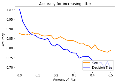
Note how the decision tree result drops quickly. This is because even though we are just shifting the original data just a tiny bit, because it’s so overfitted it quickly starts to misclassify data.

Which do you think is the better model?

Bonus

• Write some code to plot the decision boundaries of the classifiers. To do this the easiest thing is to just generate a load of random x,y coords and use the model to generate the class. Compare that to the plot above.

Hint: Take a look at some of the other workshops.