Support Vector Machines
Support Vector Machines
Welcome! This workshop is from Winder.ai. Sign up to receive more free workshops, training and videos.
If you remember from the video training, SVMs are classifiers that attemt to maximise the separation between classes, no matter what the distribution of the data. This means that they can sometimes fit noise more than they fit the data.
But because they are aiming to separate classes, they do a really good job at optimising for accuracy. Let’s investigate this below.
# Usual imports
import os
import pandas as pd
import matplotlib.pyplot as plt
import numpy as np
from IPython.display import display
from sklearn import datasets
from sklearn import preprocessing
# import some data to play with
iris = datasets.load_iris()
feat = iris.feature_names
X = iris.data[:, :2]  # we only take the first two features. We could
                      # avoid this ugly slicing by using a two-dim dataset
y = iris.target
y[y != 0] = 1 # Only use two targets for now
colors = "bry"

# standardize
X = preprocessing.StandardScaler().fit_transform(X)
from sklearn.svm import SVC
# Create a linear SVM
svm_clf = SVC(kernel='linear', C=float("inf")).fit(X, y)
# A fairly complicated function to plot the decision boundary and separation found by a liner SVM.
def plot_svc_decision_boundary(svm_clf, xmin, xmax):
    w = svm_clf.coef_[0]
    b = svm_clf.intercept_[0]

    # At the decision boundary, w0*x0 + w1*x1 + b = 0
    # => x1 = -w0/w1 * x0 - b/w1
    x0 = np.linspace(xmin, xmax, 200)
    decision_boundary = -w[0]/w[1] * x0 - b/w[1]

    margin = 1/w[1]
    gutter_up = decision_boundary + margin
    gutter_down = decision_boundary - margin

    svs = svm_clf.support_vectors_
    plt.scatter(svs[:, 0], svs[:, 1], s=180, facecolors='#FFAAAA')
    plt.plot(x0, decision_boundary, "k-", linewidth=2, label="SVM")
    plt.plot(x0, gutter_up, "k--", linewidth=2)
    plt.plot(x0, gutter_down, "k--", linewidth=2)

# Usual plotting related stuff.
plot_svc_decision_boundary(svm_clf, -2, 2)
plt.scatter(X[y == 0, 0], X[y == 0, 1],
            color='red', marker='o', label='setosa')
plt.scatter(X[y != 0, 0], X[y != 0, 1],
            color='blue', marker='x', label='not setosa')
plt.axis([-2, 2.5, -3, 3.5])
plt.xlabel(feat[0])
plt.ylabel(feat[1])
plt.legend(loc='upper left')
plt.show()
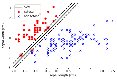
Note how the SVM has maximised the separation between the classes and also allowed some datapoints to enter within the boundary. The SVM parameter C is a penalty parameter that specifies whether it should force the separation of the classes (C=inf) or allow some points to be misclassified to obtain a better fit (C=small).
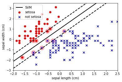
Let’s allow some level of misclassification to get a better (IMO) decision boundary:
svm_clf = SVC(kernel='linear', C=1.0).fit(X, y)
plot_svc_decision_boundary(svm_clf, -2, 2)
plt.scatter(X[y == 0, 0], X[y == 0, 1],
            color='red', marker='o', label='setosa')
plt.scatter(X[y != 0, 0], X[y != 0, 1],
            color='blue', marker='x', label='not setosa')
plt.axis([-2, 2.5, -3, 3.5])
plt.xlabel(feat[0])
plt.ylabel(feat[1])
plt.legend(loc='upper left')
plt.show()
Kernel Trick
Remember that it is possible to transform the input data without compromising the integrity of the data. The transformation simply needs to be invertible. The “kernel trick” is a method to transform the data by a complex (invertible) function to allow more complex decision boundaries.
When we preform this trick with SVMs the result is a Kernel SVM. In the next example we choose a radial basis function for our kernel. This is basically a multi-dimensional gaussian. We specify the width of this kernel with the gamma parameter. Smaller values of gamma will produce more complex boundaries (less smoothing).
from sklearn.svm import SVC
# This is a Support vector machine with a "radial basis function" kernel.
# One issue with SVMs is that they are quite complex to tune, because of all the different parameters.
rbf_svc = SVC(kernel='rbf', gamma=0.7, C=float('inf')).fit(X, y)
from matplotlib.colors import ListedColormap

# A fancy method to plot the decision regions of complex decision boundaries
def plot_decision_regions(X, y, classifier, test_idx=None, resolution=0.02, labels=['setosa', 'not setosa'], X_plot=None):

    if X_plot is None:
        X_plot = X

    # setup marker generator and color map
    markers = ('s', 'x', 'o', '^', 'v')
    colors = ('red', 'blue', 'lightgreen', 'gray', 'cyan')
    cmap = ListedColormap(colors[:len(np.unique(y))])

    # plot the decision surface
    x1_min, x1_max = X[:, 0].min() - 1, X[:, 0].max() + 1
    x2_min, x2_max = X[:, 1].min() - 1, X[:, 1].max() + 1
    xx1, xx2 = np.meshgrid(np.arange(x1_min, x1_max, resolution),
                         np.arange(x2_min, x2_max, resolution))
    Z = classifier.predict(np.array([xx1.ravel(), xx2.ravel()]).T)
    Z = Z.reshape(xx1.shape)
    plt.contourf(xx1, xx2, Z, alpha=0.4, cmap=cmap)
    plt.xlim(xx1.min(), xx1.max())
    plt.ylim(xx2.min(), xx2.max())

    # plot all samples
    X_test, y_test = X[test_idx, :], y[test_idx]
    for idx, cl in enumerate(np.unique(y)):
        plt.scatter(x=X[y == cl, 0], y=X[y == cl, 1],
                    alpha=0.8, c=cmap(idx),
                    marker=markers[idx], label=labels[cl])

    # highlight test samples
    if test_idx:
        X_test, y_test = X[test_idx, :], y[test_idx]
        plt.scatter(X_test[:, 0], X_test[:, 1], c='',
                alpha=1.0, linewidth=1, marker='o',
                s=55, label='test set')
plot_decision_regions(X=X, y=y, classifier=rbf_svc)
plt.xlabel(feat[0])
plt.ylabel(feat[1])
plt.legend(loc='upper left')

plt.axis([-2, 2.5, -3, 3.5])
plt.show()
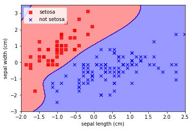
Note how insane that decision boundary is. To the extent that the algorithm has “invented” a blue decision region at the top left where there is absolutely no evidence that it should be there. This is the risk of choosing such arbitrary decision boundaries; arbitrary results.