Linear Regression

Welcome! This workshop is from Winder.ai. Sign up to receive more free workshops, training and videos.

Regression is a traditional task from statistics that attempts to fit model to some input data to predict the numerical value of an output. The data is assumed to be continuous.

The goal is to be able to take a new observation and predict the output with minmal error. Some examples might be “what will next quater’s profits be?” and “how many widgets do we need to stock in order to fulfil demand?”.

For these questions we need real, numerical answers. But we can also use regression-like models as a basis for classification too, and in fact there are many algorithms that are based upon this.

# Usual imports
import os
import pandas as pd
import matplotlib.pyplot as plt
import numpy as np
from IPython.display import display

np.random.seed(42)  # To ensure we get the same data every time.
X = 2 * np.random.rand(50, 1)
y = 8 + 6 * X + np.random.randn(50, 1)

Since we’ve only got a one dimensional input (that doesn’t happen very often!) let’s plot the data (input vs. output).

When we plot observations on an x-y scale, this is known as a scatter plot.

Tasks

• Try changing the colours, markers and labels of the plot (you may need to look at the documentation for this)

plt.scatter(X, y, color='red', marker='o')
plt.xlabel('x')
plt.ylabel('y')
plt.tight_layout()
plt.axis([0, 2, 8, 22])
plt.show()

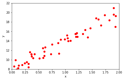
Here we can see the x and y values are clearly correlated. Let’s estimate that correlation..

cc = np.corrcoef(X, y, rowvar=0)
print("Correlation coefficient: %.2f" % cc[0,1])

Correlation coefficient: 0.97

0.97 is a huge correlation.

Now, remember that there is a closed solution to find the optimal MSE for a given data. It’s called the Normal equation.

$$ \begin{align} \hat{w}=\left(\mathbf{x}^T\cdot\mathbf{x}\right)^{-1} \cdot \mathbf{x}^T \cdot \mathbf{y} \end{align} $$

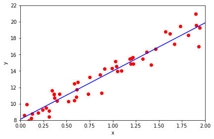
Let’s write that equation in numpy, then plot the result…

X_b = np.c_[np.ones((50, 1)), X] # add x0 = 1 to each instance (the intercept term, c, in y = mx + c)
w = np.linalg.inv(X_b.T.dot(X_b)).dot(X_b.T).dot(y) # Implementation of the closed form solution.
print(w) # Print the final values of the weights (intercept and slope, in this case)

[[ 8.09668927]
 [ 5.888283  ]]

X_new = np.array([[0], [2]])  # Create two x points to be able to draw the line
y_predict = np.array([w[0], X_new[1]*w[1] + w[0]]) # Predict the y values for these two points.

# Plot the scatter plot
plt.scatter(X, y, color='red', marker='o')
plt.plot(X_new, y_predict, "b-")
plt.xlabel('x')
plt.ylabel('y')
plt.tight_layout()
plt.axis([0, 2, 8, 22])
plt.show()

Regression in sklearn

Now doing all this math by hand is grand, but 95% of the time, you will be more productive by using a library, especially during early phases of a data science project.

So let’s reproduce the previous regression in sklearn…

from sklearn.linear_model import LinearRegression
lin_reg = LinearRegression()
lin_reg.fit(X, y)
lin_reg.intercept_, lin_reg.coef_
# Results should be the same as before...

(array([ 8.09668927]), array([[ 5.888283]]))