Linear Classification
Linear Classification
Welcome! This workshop is from Winder.ai. Sign up to receive more free workshops, training and videos.
We learnt that we can use a linear model (and possibly gradient descent) to fit a straight line to some data. To do this we minimised the mean-squared-error (often known as the optimisation/loss/cost function) between our prediction and the data.
It’s also possible to slightly change the optimisation function to fit the line to separate classes. This is called linear classification.
# Usual imports
import os
import pandas as pd
import matplotlib.pyplot as plt
import numpy as np
from IPython.display import display
from sklearn import datasets
from sklearn import preprocessing
# import some data to play with
iris = datasets.load_iris()
feat = iris.feature_names
X = iris.data[:, :2]  # we only take the first two features. We could
                      # avoid this ugly slicing by using a two-dim dataset
y = iris.target
y[y != 0] = 1 # Only use two targets for now
colors = "bry"

# standardize
X = preprocessing.StandardScaler().fit_transform(X)

# plot data
plt.scatter(X[y == 0, 0], X[y == 0, 1],
            color='red', marker='o', label='setosa')
plt.scatter(X[y != 0, 0], X[y != 0, 1],
            color='blue', marker='x', label='not setosa')

plt.xlabel(feat[0])
plt.ylabel(feat[1])
plt.legend(loc='upper left')
plt.show()
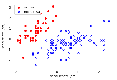
We can visually see that there is a clear demarcation between the classes.
We theorise that we should be able to make a robust classifier with a simple linear model.
Let’s do that with the classsification version of the stochastic gradient descent algorithm
from sklearn.linear_model.SGDClassifier…
from sklearn.linear_model import SGDClassifier
clf = SGDClassifier(loss="squared_loss", learning_rate="constant", eta0=0.01, max_iter=10, penalty=None).fit(X, y)
plt.scatter(X[y == 0, 0], X[y == 0, 1],
            color='red', marker='o', label='setosa')
plt.scatter(X[y != 0, 0], X[y != 0, 1],
            color='blue', marker='x', label='not setosa')

# Plot the three one-against-all classifiers
xmin, xmax = plt.xlim()
ymin, ymax = plt.ylim()
coef = clf.coef_
intercept = clf.intercept_

def plot_hyperplane(c, color, label):
    def line(x0):
        return (-(x0 * coef[c, 0]) - intercept[c]) / coef[c, 1]

    plt.plot([xmin, xmax], [line(xmin), line(xmax)],
             ls="--", color=color, label=label)


plot_hyperplane(0, 'b', "L2 loss")

plt.xlabel(feat[0])
plt.ylabel(feat[1])
plt.legend(loc='upper left')
plt.show()
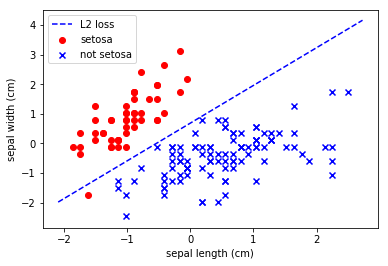
Not too bad.
Tasks
- Try altering the values of eta and the number of iterations
We don’t use any regularization here, because we only have two features. This would be far more important when we had multiple features.