K-NN For Classification
K-NN For Classification
Welcome! This workshop is from Winder.ai. Sign up to receive more free workshops, training and videos.
In a previous workshop we investigated how the nearest neighbour algorithm uses the concept of distance as a similarity measure.
We can also use this concept of similarity as a classification metric. I.e. new observations will be classified the same as its neighbours.
This is accomplished by finding the most similar observations and setting the predicted classification as some combination of the k-nearest neighbours. (e.g. the most common)
This time, let’s use a classification dataset like the iris dataset and
let’s use the inbuilt k-NN implementation in sklearn.
# Usual imports
import os
import pandas as pd
import matplotlib.pyplot as plt
import numpy as np
from IPython.display import display
from sklearn import datasets
from sklearn import neighbors

# import some data to play with
iris = datasets.load_iris()
X = iris.data[:, :2]  # we only take the first two features. We could
                      # avoid this ugly slicing by using a two-dim dataset
y = iris.target
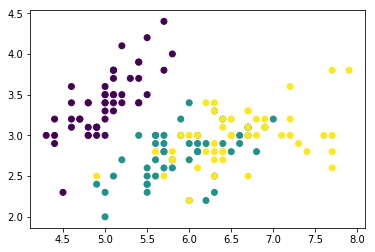
# Quick plot to see what we're dealing with
plt.scatter(X[:,0], X[:,1], c=y)
plt.show()
Now let’s write a fancy method to plot the decision boundaries…
from matplotlib.colors import ListedColormap

def plot_decision_regions(X, y, classifier, resolution=0.02):
    # setup marker generator and color map
    markers = ('s', 'x', 'o', '^', 'v')
    colors = ('red', 'blue', 'lightgreen', 'gray', 'cyan')
    cmap = ListedColormap(colors[:len(np.unique(y))])
    cmap_bold = ListedColormap(['#FF0000', '#00FF00', '#0000FF'])

    # plot the decision surface
    x1_min, x1_max = X[:, 0].min() - 1, X[:, 0].max() + 1
    x2_min, x2_max = X[:, 1].min() - 1, X[:, 1].max() + 1
    xx1, xx2 = np.meshgrid(np.arange(x1_min, x1_max, resolution),
                         np.arange(x2_min, x2_max, resolution))
    Z = classifier.predict(np.array([xx1.ravel(), xx2.ravel()]).T)
    Z = Z.reshape(xx1.shape)
    plt.contourf(xx1, xx2, Z, alpha=0.4, cmap=cmap)
    plt.xlim(xx1.min(), xx1.max())
    plt.ylim(xx2.min(), xx2.max())

    plt.scatter(X[:, 0], X[:, 1], c=y, cmap=cmap_bold)
figure = plt.figure(figsize=(12, 6))
n_neighbours = [1, 20]
i = 1
for n in n_neighbours:
    clf = neighbors.KNeighborsClassifier(n, weights='distance')
    clf.fit(X, y)
    ax = plt.subplot(1, len(n_neighbours), i)
    i += 1

    plot_decision_regions(X=X, y=y, classifier=clf)
    ax.set_xticks(())
    ax.set_yticks(())
    plt.title(str(n) + '-NN')

plt.show()
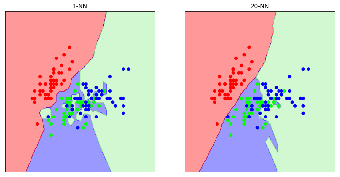
As we can see, when we only pick a single neighbour for classification purposes, we end up with a very complex decision boundary. If we were to perform validation on this classifier we would probably see that it has poor performance; we have overfit.
Generally, as you increase the value of k, the decision boundary becomes smoother.
But beware. You must pick a value of k to avoid ties (i.e. odd) and it must be coprime (to allow all classes a chance to vote). See the training videos for more information.
Tasks
- Try plotting validation curves on this dataset for different values of k