Introduction to Gradient Descent

Welcome! This workshop is from Winder.ai. Sign up to receive more free workshops, training and videos.

For only a few algorithms an analytical solution exists. For example, we can use the Normal Equation to solve a linear regression problem directly.

However, for most algorithms we rely cannot solve the problem analytically; usually because it’s impossible to solve the equation. So instead we have to try something else.

Gradient Descent is the idea that we can “roll down” the error curve. Let’s plot an error curve for a simple model to make this more concrete.

# Usual imports
import os
import pandas as pd
import matplotlib.pyplot as plt
import numpy as np
from IPython.display import display

np.random.seed(42)  # To ensure we get the same data every time.
X = np.random.normal(loc=2, scale=0.3, size=(1000,1))
def plot_grid():
    for m in [1.5, 2.5]:
        plt.plot([m,m], [0, 1], 'k--')
    plt.plot([2,2], [0, 1], 'r--')
plt.plot(X, np.random.rand(len(X),1), 'x')
plot_grid()
plt.xlim([1,3])
plt.ylim([0,1])
plt.yticks([])
plt.show()

def mse(X, m):
    return np.sum(np.square((m - X)))/len(X)

m_values = np.linspace(1, 3, 40)
err = [mse(X, m) for m in m_values]
plt.plot(m_values, err)
plot_grid()
plt.xlim([1,3])
plt.ylim([0,1])
plt.show()

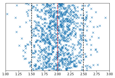
The above plots show some one-dimensional normally distributed data around 2.0. We can estimate the location of line that represents the most probable value with the mean. But imagine we couldn’t calculate the mean for some reason.

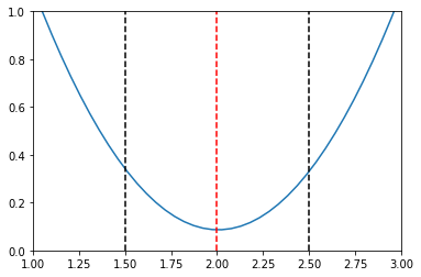
What we can do is slide a range of prospective mean estimates across the data and calculate the mean squared error at each point. The value of the mean squared error for each prospective mean is shown in the second plot.

The red line represents the point at which the error is lowest. Around this point there is a convex slope.

Gradient descent works by calculating the slope of the error at a particular point. It then moves the parameters so that we move down that slope. Eventually we end up at the bottom.

So how do we calculate the gradient? With differential calculus.

Using Gradient Descent

Below is the matrix form of the partial derivative of the mean squared error.

We can use this equation to update our prospective parameters, known as weights, and iterate towards the bottom of the error surface. (I say surface, not curve, because generally we’re working in more than one dimension).

$$ \nabla_{\mathbf{w}} MSE(\mathbf{w}) = \frac{2}{m}\mathbf{x}^T \cdot (\mathbf{x} \cdot \mathbf{w} - \mathbf{y}) $$

Where \(m\) is the number of observations.

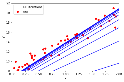
If we used the equation above to update our weights directly, then we actually end up jumping straight to the bottom. However, we don’t generally want to move there in one hop. We want to take it slowly to ensure that we really are still going down the slope.

So instead, we weight the update by a small fraction to slow it down.

So once you have calculated the gradient using the equation above, update the current value of \(\mathbf{w}\) by

$$ \mathbf{w} = \mathbf{w} - \eta \nabla_{\mathbf{w}} $$

np.random.seed(42)  # To ensure we get the same data every time.
X = 2 * np.random.rand(50, 1)
X_b = np.c_[np.ones((50, 1)), X] # add x0 = 1 to each instance (the intercept term, c, in y = mx + c)
y = 8 + 6 * X + np.random.randn(50, 1)

eta = 0.1 # learning rate
n_iterations = 10 # number of iterations
m=len(X) # number of samples

w = np.random.randn(2,1) # random initialization of parameters
w_old = []
for iteration in range(n_iterations):
    gradients = 2/m * X_b.T.dot(X_b.dot(w) - y)
    w = w - eta * gradients
    w_old.append(w)

X_new = np.array([[0], [2]])  # Create two x points to be able to draw the line
plt.scatter(X, y,
            color='red', marker='o', label='raw')
for w_i in w_old:
    y_predict = np.array([w_i[0], X_new[1]*w_i[1] + w_i[0]])
    plt.plot(X_new, y_predict, "b-")
plt.plot(X_new, y_predict, "b-", label='GD iterations')
plt.xlabel('x')
plt.ylabel('y')
plt.legend(loc='upper left')
plt.tight_layout()
plt.axis([0, 2, 8, 22])
plt.show()

### Tasks:

• What happens when you alter the learning rate?
• What happens when you alter the number of iterations?

And of course, this is already implemented in sklearn under SGDRegressor. Feel free to check that this produces the same result if you wish.