Fast Time-Series Filters in Python

Time-series (TS) filters are often used in digital signal processing for distributed acoustic sensing (DAS). The goal is to remove a subset of frequencies from a digitised TS signal. To filter a signal you must touch all of the data and perform a convolution. This is a slow process when you have a large amount of data. The purpose of this post is to investigate which filters are fastest in Python.

Parallel Processing

The data must be streamed through the filter because the filter contains state. The next filtering step depends on the previous result and the current state of the filter. It is a Markov process.

This makes it difficult to parallelise. If you have a one-dimensional TS, you cannot split it to run on two threads, because of the Markov property. In two-dimensional TS signals, like stereo audio for example, you could split the channels and run the filters on separate threads. Note that there are also packages that provide multi-threaded numpy and scipy installations like Intel’s Python distribution.

Filter Type

There are two types of digital TS filter: finite impulse response (FIR) and infinite impulse response (IIR). If you filtered a signal that had a spike (an impulse) in it, the IIR filter would oscillate infinitely, whereas FIRs would ring for a short period of time. IIR filters are recursive.

FIR and IIR filters are defined by the number of observations they convolve over, often called the order or number of taps. Because IIR filters are recursive, they can perform as well as FIR filters with far fewer taps. This should mean that IIR filters are faster given the same filtering requirements. The downside is that they can be unstable (because of the feedback loop) and they alter the phase of the signal in a non-linear way (e.g. high frequencies and low-frequencies could be separated in time when they go through the filter).

SciPy

scipy has a range of methods to help design filter parameters and perform the filtering. It uses numpy under-the-hood, so the underlying convolutions should be performant. Let us start by defining some common parameters.

import numpy as np
import scipy as sp
import scipy.signal as signal
import matplotlib.pyplot as plt
import timeit

sampling_frequency = 10000.0        # Sampling frequency in Hz
nyq = sampling_frequency * 0.5  # Nyquist frequency
passband_frequencies = (5.0, 150.0)  # Filter cutoff in Hz
stopband_frequencies = (1.0, 1000.0)
max_loss_passband = 3 # The maximum loss allowed in the passband
min_loss_stopband = 30 # The minimum loss allowed in the stopband
x = np.random.random(size=(5000, 12500)) # Random data to be filtered

Designing an IIR Filter

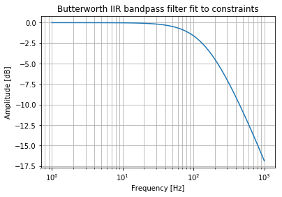
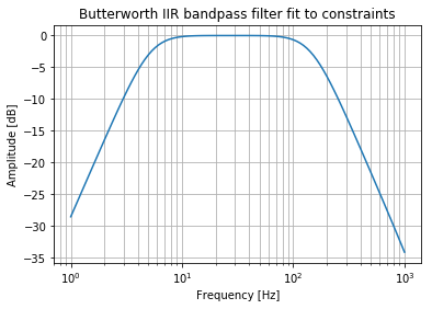
Now we need to design the filter. scipy has several helper methods that allow us to take our specifications and recommend the order of the filter. In the code below we design a bandpass Butterworth IIR filter. The result is a filter with an order 3.

order, normal_cutoff = signal.buttord(passband_frequencies, stopband_frequencies, max_loss_passband, min_loss_stopband, fs=sampling_frequency)
iir_b, iir_a = signal.butter(order, normal_cutoff, btype="bandpass", fs=sampling_frequency)
w, h = signal.freqz(iir_b, iir_a, worN=np.logspace(0, 3, 100), fs=sampling_frequency)
plt.semilogx(w, 20 * np.log10(abs(h)))
plt.title('Butterworth IIR bandpass filter fit to constraints')
plt.xlabel('Frequency [Hz]')
plt.ylabel('Amplitude [dB]')
plt.grid(which='both', axis='both')
plt.show()

Designing a FIR Filter

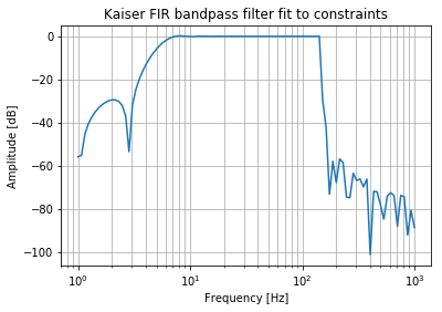
Now let us use the same parameters to design an FIR filter. This is a bandpass Kaiser FIR filter. 5Hz is a low cutoff for a signal that has a sampling rate of 10 kHz. The resulting filter design has an order of approximately 2200.

This makes sense because the filter is not recursive. It has to directly observe 5Hz signals in order to filter them out. In other words we need at least 10000 / 5 = 2000 observations to see a 5 Hz signal.

The filter attenuation performance is also poor, when compared to the Butterworth. But at least there won’t be any nonlinear phase changes.

nyq_cutoff = (passband_frequencies[0] - stopband_frequencies[0]) / nyq
N, beta = signal.kaiserord(min_loss_stopband, nyq_cutoff)
fir_b = signal.firwin(N, passband_frequencies, window=('kaiser', beta), fs=sampling_frequency, pass_zero=False, scale=False)
fir_a = 1.0
w, h = signal.freqz(fir_b, fir_a, worN=np.logspace(0, 3, 100), fs=sampling_frequency)
plt.semilogx(w, 20 * np.log10(abs(h)))
plt.title('Kaiser FIR bandpass filter fit to constraints')
plt.xlabel('Frequency [Hz]')
plt.ylabel('Amplitude [dB]')
plt.grid(which='both', axis='both')
plt.show()

scipy.signal.lfilter Performance

Now I will test the performance of the scipy.signal.lfilter function on these two filters. I expect the FIR to be slow, because it has to perform so many more computations. I.e. for each channel there would be 2000 x len(signal) multiplications, where as for the IIR there would only be 3 x len(signal). numpy may be able to optimise the calculation, but I would still expect around two orders of magnitude of difference.

print("IIR time = {}".format(timeit.timeit(lambda: signal.lfilter(iir_b, iir_a, x, axis=1), number=1)))
print("FIR time = {}".format(timeit.timeit(lambda: signal.lfilter(fir_b, fir_a, x, axis=1), number=1)))

IIR time = 0.8159449380000297
FIR time = 57.0915518339998

These result show what I expected. When you need to filter low frequencies, IIRs are dramatically more efficient.

Improving IIR Filter Performance

The scipy lfilter function uses a lot of compiled C. It is unlikely that I would be able to improve the performance of the code underlying lfilter. But what about if we try using two smaller filters?

Let me first run the baseline again to get a better average.

print("Average baseline IIR time = {}".format(timeit.timeit(lambda: signal.lfilter(iir_b, iir_a, x, axis=1), number=10) / 10))

Average baseline IIR time = 0.6693926614000703

Now let me design two new order 1 filters.

b_hp, a_hp = signal.butter(1, normal_cutoff[0], btype="highpass", fs=sampling_frequency)
w, h = signal.freqz(b_hp, a_hp, worN=np.logspace(0, 3, 100), fs=sampling_frequency)
plt.semilogx(w, 20 * np.log10(abs(h)))
plt.title('Butterworth IIR bandpass filter fit to constraints')
plt.xlabel('Frequency [Hz]')
plt.ylabel('Amplitude [dB]')
plt.grid(which='both', axis='both')
plt.show()

b_lp, a_lp = signal.butter(1, normal_cutoff[1], btype="lowpass", fs=sampling_frequency)
w, h = signal.freqz(b_lp, a_lp, worN=np.logspace(0, 3, 100), fs=sampling_frequency)
plt.semilogx(w, 20 * np.log10(abs(h)))
plt.title('Butterworth IIR bandpass filter fit to constraints')
plt.xlabel('Frequency [Hz]')
plt.ylabel('Amplitude [dB]')
plt.grid(which='both', axis='both')
plt.show()

def two_filters(x):
  y = signal.lfilter(b_hp, a_hp, x, axis=1)
  z = signal.lfilter(b_lp, a_lp, y, axis=1)
  return z

print("Average two filter time = {}".format(timeit.timeit(lambda: two_filters(x), number=10) / 10))

Average two filter time = 0.8258036216999244

Doh. That’s a bit slower. We can combine those filters with a convolve. Let’s try that.

Combining Separate Filters

Remember that filtering is a convolution operation. And convolution is associative. I.e. imagine two filters, a and b, a signal x and a convolution C. Filtering a signal x by filter a is C(x, a). Using two filters: C( C(x, a), b). Which is the same as: C(x, C(a, b)). Hence, convolve the filters together first and you end up with a single filter.

a = sp.convolve(a_lp, a_hp)
b = sp.convolve(b_lp, b_hp)
print("Average combined filter time = {}".format(timeit.timeit(lambda: signal.lfilter(b, a, x, axis=1), number=10) / 10))

Average combined filter time = 0.42798648080006385

Cool, that’s faster. But I suspect it is the same as just using an order of 2 in the filter design.

b, a = signal.butter(2, normal_cutoff, btype="bandpass", fs=sampling_frequency)
w, h = signal.freqz(b, a, worN=np.logspace(0, 3, 100), fs=sampling_frequency)
plt.semilogx(w, 20 * np.log10(abs(h)))
plt.title('Butterworth IIR bandpass filter fit to constraints')
plt.xlabel('Frequency [Hz]')
plt.ylabel('Amplitude [dB]')
plt.grid(which='both', axis='both')
plt.show()

print("Average order 2 IIR filter time = {}".format(timeit.timeit(lambda: signal.lfilter(b, a, x, axis=1), number=10) / 10))

Average order 2 IIR filter time = 0.44366712920000284

Yep. There we go. Individual highpass/lowpass filter design has the same performance as a bandpass of the same order (1 + 1 in this example). Individual design could be useful if you have different requirements.

Combining IIR and FIR Filters

What about using an IIR filter for the HP, then an FIR for the LP? I will pick an order that produces the same results at 1000 Hz as the IIR filter (approximately -35 dB).

b_fir_lp = signal.firwin(20, passband_frequencies[1], fs=sampling_frequency, pass_zero=True, scale=True)
w, h = signal.freqz(fir_b, fir_a, worN=np.logspace(0, 3, 100), fs=sampling_frequency)
plt.semilogx(w, 20 * np.log10(abs(h)))
plt.title('Kaiser FIR bandpass filter fit to constraints')
plt.xlabel('Frequency [Hz]')
plt.ylabel('Amplitude [dB]')
plt.grid(which='both', axis='both')
plt.show()

def iir_fir(x):
  y = signal.lfilter(b_hp, a_hp, x, axis=1)
  z = signal.lfilter(b_fir_lp, 1.0, y, axis=1)
  return z

print("Average two filter time = {}".format(timeit.timeit(lambda: iir_fir(x), number=10) / 10))

Average two filter time = 1.9922046989999216

No, still very poor.

Conclusions

scipy and numpy have been optimised to the point where it is unlikely that you can improve performance by writing your own filtering methods. This means that filter performance is entirely defined by your filter definition and the order of the filter. A higher order means more multiplications.

So if you are primarily interested in performance, use IIR filters and keep the order as low as possible. If you have different requirements for the high or low cutoff frequencies then design them independently and combine.

In terms of speeding up scipy performance, then use multiple threads to filter separate channels or use a different implementation of Python or scipy to leverage multi-theaded support.