Entropy Based Feature Selection
Entropy Based Feature Selection
Welcome! This workshop is from Winder.ai. Sign up to receive more free workshops, training and videos.
One simple way to evaluate the importance of features (something we will deal with later) is to calculate the entropy for prospective splits.
In this example, we will look at a real dataset called the “mushroom dataset”. It is a large collection of data about poisonous and edible mushrooms.
Attribute Information: (classes: edible=e, poisonous=p) 1. cap-shape: bell=b,conical=c,convex=x,flat=f, knobbed=k,sunken=s 2. cap-surface: fibrous=f,grooves=g,scaly=y,smooth=s 3. cap-color: brown=n,buff=b,cinnamon=c,gray=g,green=r, pink=p,purple=u,red=e,white=w,yellow=y 4. bruises?: bruises=t,no=f 5. odor: almond=a,anise=l,creosote=c,fishy=y,foul=f, musty=m,none=n,pungent=p,spicy=s
# Load the data with a library called pandas. Pandas is very cool, and we will be using it a lot.
import pandas as pd
import numpy as np

# We're going to use the display module to embed some outputs
from IPython.display import display

# Read data using Pandas from the UCI data repository.
feature_names = ["poisonous", "cap-shape", "cap-surface", "cap-color", "bruises?", "odor", "gill-attachment", "gill-spacing", "gill-size", "gill-color", "stalk-shape", "stalk-root", "stalk-surface-above-ring", "stalk-surface-below-ring", "stalk-color-above-ring", "stalk-color-below-ring", "veil-type", "veil-color", "ring-number", "ring-type", "spore-print-color", "population", "habitat"]
X = pd.read_csv("https://archive.ics.uci.edu/ml/machine-learning-databases/mushroom/agaricus-lepiota.data", header=0, names=feature_names)
y = X["poisonous"]                      # Select target label
X.drop(['poisonous'], axis=1, inplace=True)   # Remove target label from dataset
display(X.head())                       # Show some data

y = y.map({"e": 0, "p": 1})             # Mapping the classes to zeros and ones, not strictly necessary.
display(y.head())
| cap-shape | cap-surface | cap-color | bruises? | odor | gill-attachment | gill-spacing | gill-size | gill-color | stalk-shape | ... | stalk-surface-below-ring | stalk-color-above-ring | stalk-color-below-ring | veil-type | veil-color | ring-number | ring-type | spore-print-color | population | habitat | |
|---|---|---|---|---|---|---|---|---|---|---|---|---|---|---|---|---|---|---|---|---|---|
| 0 | x | s | y | t | a | f | c | b | k | e | ... | s | w | w | p | w | o | p | n | n | g |
| 1 | b | s | w | t | l | f | c | b | n | e | ... | s | w | w | p | w | o | p | n | n | m |
| 2 | x | y | w | t | p | f | c | n | n | e | ... | s | w | w | p | w | o | p | k | s | u |
| 3 | x | s | g | f | n | f | w | b | k | t | ... | s | w | w | p | w | o | e | n | a | g |
| 4 | x | y | y | t | a | f | c | b | n | e | ... | s | w | w | p | w | o | p | k | n | g |
5 rows × 22 columns
0    0
1    0
2    1
3    0
4    0
Name: poisonous, dtype: int64
# This is the entropy method we defined in the Entropy workshop
def entropy(y):
    probs = [] # Probabilities of each class label
    for c in set(y): # Set gets a unique set of values. We're iterating over each value
        num_same_class = sum(y == c)  # Remember that true == 1, so we can sum.
        p = num_same_class / len(y) # Probability of this class label
        probs.append(p)
    return np.sum(-p * np.log2(p) for p in probs)

# What is the entropy of the entire set?
print("Entire set entropy = %.2f" % entropy(y))
Entire set entropy = 1.00
# Let's write some functions that calculates the entropy after splitting on a particular value

def class_probability(feature, y):
    """Calculates the proportional length of each value in the set of instances"""
    # This is doc string, used for documentation
    probs = []
    for value in set(feature):
        select = feature == value # Split by feature value into two classes
        y_new = y[select]         # Those that exist in this class are now in y_new
        probs.append(float(len(y_new))/len(X))  # Convert to float, because ints don't divide well
    return probs

def class_entropy(feature, y):
    """Calculates the entropy for each value in the set of instances"""
    ents = []
    for value in set(feature):
        select = feature == value # Split by feature value into two classes
        y_new = y[select]         # Those that exist in this class are now in y_new
        ents.append(entropy(y_new))
    return ents

def proportionate_class_entropy(feature, y):
    """Calculatates the weighted proportional entropy for a feature when splitting on all values"""
    probs = class_probability(feature, y)
    ents = class_entropy(feature, y)
    return np.sum(np.multiply(probs, ents)) # Information gain equation
# Let's try calculating the entropy after splitting by all the values in "cap-shape"
new_entropy = proportionate_class_entropy(X["cap-shape"], y)
print("Information gain of %.2f" % (entropy(y) - new_entropy))
# Should be an information gain of 0.05
Information gain of 0.05
# Now let's try doing the same when splitting based upon all values of "odor"
new_entropy = proportionate_class_entropy(X["odor"], y)
print("Information gain of %.2f" % (entropy(y) - new_entropy))
# Should be an information gain of 0.91
Information gain of 0.91
Clearly, if we were thinking about looking at individual features, then odor would be a far better prospect than cap-shape.
This is cool. You have manually implemented a Decision Tree! Well done! Later on we’ll use a library to do this sort of thing.
Which Feature Produces the Best Split?
We can repeat this process for all features. The best split is the one with the highest information gain.
for c in X.columns:
    new_entropy = proportionate_class_entropy(X[c], y)
    print("%s %.2f" % (c, entropy(y) - new_entropy))
cap-shape 0.05
cap-surface 0.03
cap-color 0.04
bruises? 0.19
odor 0.91
gill-attachment 0.01
gill-spacing 0.10
gill-size 0.23
gill-color 0.42
stalk-shape 0.01
stalk-root 0.13
stalk-surface-above-ring 0.28
stalk-surface-below-ring 0.27
stalk-color-above-ring 0.25
stalk-color-below-ring 0.24
veil-type 0.00
veil-color 0.02
ring-number 0.04
ring-type 0.32
spore-print-color 0.48
population 0.20
habitat 0.16
Plotting
Throughout data science, results are more intruitive to reason about if you present the data or the results in different media.
Plotting is used for everything; investigating data through to presenting results.
You should become familiar with plotting data; below we go through a fairly comprehensive example.
# Matplotlib is _the_ plotting library for python. Most other tools are based
# upon matplot lib. We will use others as appropriate in the future (mainly
# pandas's helpers)
import matplotlib.pyplot as plt

colours = 'bgrcmk'  # An array of colours used during plotting later on.

def plot_entropy(probability, entropy, labels):
    """Graphical representation of entropy when splitting on each value"""

    # Some complex calculations to get the centre of the bars
    positions = np.array([0])
    positions = np.concatenate((positions, np.cumsum(probability)[:-1]))
    positions += np.divide(probability, 2)

    # Plot bars with colours
    plt.bar(positions, entropy, width=probability, color=colours[:len(probability)])

    # Set limits
    plt.ylim([0, 1])
    plt.xlim([0, 1])

    # Labels
    plt.ylabel("Entropy")
    plt.xlabel("Probability")

    # If labels are provided, plot some text
    if labels:
        props = dict(boxstyle='round', facecolor='wheat', alpha=0.5)
        for i, lab in enumerate(labels):
            # Plot text
            plt.text(positions[i], 0.1, lab, fontsize=14, verticalalignment='top', bbox=props)
# Plot for "cap-shape" feature
feature = X["cap-shape"]
# Calculate probabilities and entropies
probs = class_probability(feature, y)
ents = class_entropy(feature, y)
labels = set(feature)
plot_entropy(probs, ents, labels)
plt.show() # You must run `plt.show()` at the end to show your plot.
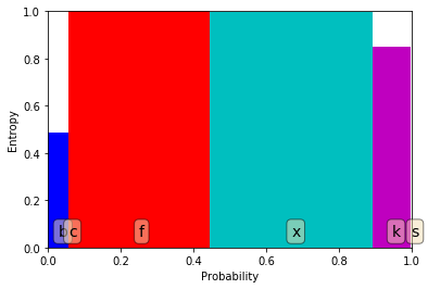
We are plotting the entropy on the y-axis and the proportion of the dataset included when performing that split on the x-axis.
This plot works well for categorical features.
The total entropy of this split is the area that is covered by all of the bars.
We can see that there isn’t much whitespace; i.e. not much information gain.
# Plot for "odor" feature
feature = X["odor"]
probs = class_probability(feature, y)
ents = class_entropy(feature, y)
labels = set(feature)
plot_entropy(probs, ents, labels)
plt.show()
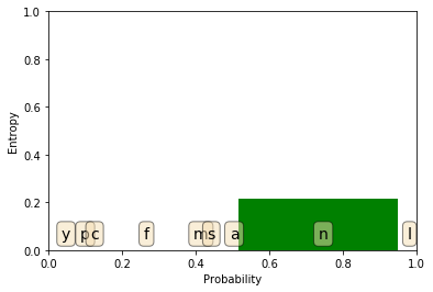
This time there is lots of whitespace. The total area is very small.
The propotionate entropy is visibly smaller.