Data Cleaning Example - Loan Data
Data Cleaning Example - Loan Data
Welcome! This workshop is from Winder.ai. Sign up to receive more free workshops, training and videos.
A huge amount of time is spent cleaning, removing, scaling data. All in an effort to squeeze a bit more performance out of the model.
The data we are using is from Kaggle, and is available in raw from from here. You will need to sign into kaggle if you want to download the full data. I’ve included just a small sample.
It is a loan dataset, showing the loans that have suffered repayment issues. There are a lot of columns and many of them are useless. Many more columns have missing data.
The goal that I set out to achieve was to attempt to predict which loans would suffer problems but we will see that it will require a lot more time to get right.
import numpy as np
import pandas as pd
import matplotlib.pyplot as plt

# Load the data
data = pd.read_csv("https://s3.eu-west-2.amazonaws.com/assets.winderresearch.com/data/loan_small.csv")
# These are the columns
data.columns
Index(['id', 'member_id', 'loan_amnt', 'funded_amnt', 'funded_amnt_inv',
       'term', 'int_rate', 'installment', 'grade', 'sub_grade', 'emp_title',
       'emp_length', 'home_ownership', 'annual_inc', 'verification_status',
       'issue_d', 'loan_status', 'pymnt_plan', 'url', 'desc', 'purpose',
       'title', 'zip_code', 'addr_state', 'dti', 'delinq_2yrs',
       'earliest_cr_line', 'inq_last_6mths', 'mths_since_last_delinq',
       'mths_since_last_record', 'open_acc', 'pub_rec', 'revol_bal',
       'revol_util', 'total_acc', 'initial_list_status', 'out_prncp',
       'out_prncp_inv', 'total_pymnt', 'total_pymnt_inv', 'total_rec_prncp',
       'total_rec_int', 'total_rec_late_fee', 'recoveries',
       'collection_recovery_fee', 'last_pymnt_d', 'last_pymnt_amnt',
       'next_pymnt_d', 'last_credit_pull_d', 'collections_12_mths_ex_med',
       'mths_since_last_major_derog', 'policy_code', 'application_type',
       'annual_inc_joint', 'dti_joint', 'verification_status_joint',
       'acc_now_delinq', 'tot_coll_amt', 'tot_cur_bal', 'open_acc_6m',
       'open_il_6m', 'open_il_12m', 'open_il_24m', 'mths_since_rcnt_il',
       'total_bal_il', 'il_util', 'open_rv_12m', 'open_rv_24m', 'max_bal_bc',
       'all_util', 'total_rev_hi_lim', 'inq_fi', 'total_cu_tl',
       'inq_last_12m'],
      dtype='object')
# There are some columns called "id". ID columns don't provide any predictive power
# so let's double check, then remove them.
display(data[["id", "member_id", "emp_title"]].head())
data.drop(['id', 'member_id'], axis=1, inplace=True)
| id | member_id | emp_title | |
|---|---|---|---|
| 0 | 1077501 | 1296599 | NaN |
| 1 | 1077430 | 1314167 | Ryder |
| 2 | 1077175 | 1313524 | NaN |
| 3 | 1076863 | 1277178 | AIR RESOURCES BOARD |
| 4 | 1075358 | 1311748 | University Medical Group |
Let’s take a deeper look at the data.
I see that there are a combination of numerical, catagorical and some messed up catagorical data here.
Let’s try and fix some of the columns as an example. In reality, you’d have to do a lot more to fix this data.
data.head()
| loan_amnt | funded_amnt | funded_amnt_inv | term | int_rate | installment | grade | sub_grade | emp_title | emp_length | ... | total_bal_il | il_util | open_rv_12m | open_rv_24m | max_bal_bc | all_util | total_rev_hi_lim | inq_fi | total_cu_tl | inq_last_12m | |
|---|---|---|---|---|---|---|---|---|---|---|---|---|---|---|---|---|---|---|---|---|---|
| 0 | 5000.0 | 5000.0 | 4975.0 | 36 months | 10.65 | 162.87 | B | B2 | NaN | 10+ years | ... | NaN | NaN | NaN | NaN | NaN | NaN | NaN | NaN | NaN | NaN |
| 1 | 2500.0 | 2500.0 | 2500.0 | 60 months | 15.27 | 59.83 | C | C4 | Ryder | < 1 year | ... | NaN | NaN | NaN | NaN | NaN | NaN | NaN | NaN | NaN | NaN |
| 2 | 2400.0 | 2400.0 | 2400.0 | 36 months | 15.96 | 84.33 | C | C5 | NaN | 10+ years | ... | NaN | NaN | NaN | NaN | NaN | NaN | NaN | NaN | NaN | NaN |
| 3 | 10000.0 | 10000.0 | 10000.0 | 36 months | 13.49 | 339.31 | C | C1 | AIR RESOURCES BOARD | 10+ years | ... | NaN | NaN | NaN | NaN | NaN | NaN | NaN | NaN | NaN | NaN |
| 4 | 3000.0 | 3000.0 | 3000.0 | 60 months | 12.69 | 67.79 | B | B5 | University Medical Group | 1 year | ... | NaN | NaN | NaN | NaN | NaN | NaN | NaN | NaN | NaN | NaN |
5 rows × 72 columns
display(set(data["emp_length"]))
data.replace('n/a', np.nan,inplace=True)
{nan,
 '9 years',
 '3 years',
 '< 1 year',
 '1 year',
 '6 years',
 '5 years',
 '4 years',
 '7 years',
 '8 years',
 '10+ years',
 '2 years'}
data.emp_length.fillna(value=0,inplace=True)
set(data["emp_length"])
{0,
 '9 years',
 '3 years',
 '< 1 year',
 '1 year',
 '6 years',
 '5 years',
 '4 years',
 '7 years',
 '8 years',
 '10+ years',
 '2 years'}
data['emp_length'].replace(to_replace='[^0-9]+', value='', inplace=True, regex=True)
data['emp_length'] = data['emp_length'].astype(int)
set(data["emp_length"])
{0, 1, 2, 3, 4, 5, 6, 7, 8, 9, 10}
I see another field called term that can be reduced to a better label
set(data['term'])
{' 36 months', ' 60 months'}
data['term'].replace(to_replace='[^0-9]+', value='', inplace=True, regex=True)
data['term'] = data['term'].astype(int)
set(data["term"])
{36, 60}
Now let’s try and define what a bad loan is…
set(data["loan_status"])
{'Charged Off', 'Current', 'Default', 'Fully Paid', 'Late (31-120 days)'}
# This indicates a bad loan. Something we want to predict
bad_indicator = data["loan_status"].isin(["Charged Off", "Default", "Late (31-120 days)"])
# Remove this from dataset
data.drop(["loan_status"], axis=1, inplace=True)
bad_indicator.value_counts()
False    820
True     179
Name: loan_status, dtype: int64
Note to future self, we have unbalanced classes here. This affects some algorithms.
# Find columns that have all nans and remove
naughty_cols = data.columns[data.isnull().sum() == len(data)]
data.drop(naughty_cols, axis=1, inplace=True)
# Any more nans?
data.columns[data.isnull().any()].tolist()
['emp_title',
 'desc',
 'mths_since_last_delinq',
 'mths_since_last_record',
 'last_pymnt_d',
 'next_pymnt_d']
# We could write some code to do this, but I'm going to do it manually for now
string_features = ["emp_title", "desc"]
data[string_features] = data[string_features].fillna(value='')
numeric_features = ["mths_since_last_delinq", "mths_since_last_record"]
data[numeric_features] = data[numeric_features].fillna(value=0)
# Any more nans, just ditch them?
just_ditch = data.columns[data.isnull().any()].tolist()
just_ditch
['last_pymnt_d', 'next_pymnt_d']
data.drop(just_ditch, axis=1, inplace=True)
Normally, we would continue improving the features until we were happy we couldn’t do any more.
When you do, remember that you will have to repeat the same steps to any new incoming data. So remember to make the pre-processing clean and pretty.
Now, let’s try and convert all those string values into numeric catagories for a tree algorithm…
from sklearn import preprocessing

selected = pd.DataFrame(data)

X = selected.apply(preprocessing.LabelEncoder().fit_transform)
X.head()
| loan_amnt | funded_amnt | funded_amnt_inv | term | int_rate | installment | grade | sub_grade | emp_title | emp_length | ... | total_rec_int | total_rec_late_fee | recoveries | collection_recovery_fee | last_pymnt_amnt | last_credit_pull_d | collections_12_mths_ex_med | policy_code | application_type | acc_now_delinq | |
|---|---|---|---|---|---|---|---|---|---|---|---|---|---|---|---|---|---|---|---|---|---|
| 0 | 32 | 32 | 32 | 0 | 6 | 119 | 1 | 6 | 0 | 10 | ... | 209 | 0 | 0 | 0 | 128 | 19 | 0 | 0 | 0 | 0 |
| 1 | 12 | 12 | 12 | 1 | 13 | 9 | 2 | 13 | 582 | 1 | ... | 71 | 0 | 27 | 4 | 79 | 44 | 0 | 0 | 0 | 0 |
| 2 | 10 | 10 | 10 | 0 | 14 | 28 | 2 | 14 | 0 | 10 | ... | 132 | 0 | 0 | 0 | 525 | 19 | 0 | 0 | 0 | 0 |
| 3 | 92 | 99 | 111 | 0 | 10 | 361 | 2 | 10 | 12 | 10 | ... | 588 | 13 | 0 | 0 | 323 | 18 | 0 | 0 | 0 | 0 |
| 4 | 14 | 14 | 14 | 1 | 9 | 13 | 1 | 9 | 744 | 1 | ... | 271 | 0 | 0 | 0 | 44 | 19 | 0 | 0 | 0 | 0 |
5 rows × 48 columns
Just for giggles, let’s fit a tree classifier and view the accuracy and feature importances.
This might give us some insight into what features are important and a baseline performance.
from sklearn.ensemble import RandomForestClassifier

clf = RandomForestClassifier(max_depth=3)
clf = clf.fit(X, bad_indicator)
from sklearn.model_selection import cross_val_score
scores = cross_val_score(clf, X, bad_indicator, cv=5, scoring='accuracy')
print("Accuracy: %0.2f (+/- %0.2f)" % (scores.mean(), scores.std()))
Accuracy: 0.95 (+/- 0.02)
Uh oh! Look how high that accuracy score is!
This should raise alarm bells.
Either the problem is super simple (and you can see the simplicity in plots) or something is not right.
Let’s look at the importances…
importances = clf.feature_importances_
std = np.std([tree.feature_importances_ for tree in clf.estimators_],
             axis=0)
indices = np.argsort(importances)[::-1]

# Print the feature ranking
print("Feature ranking:")

names = X.columns

for f in range(X.shape[1]):
    print("%d. %s (%f)" % (f + 1, names[indices[f]], importances[indices[f]]))

# Plot the feature importances of the forest
plt.figure()
plt.title("Feature importances")
plt.bar(range(X.shape[1]), importances[indices],
       color="r", yerr=std[indices], align="center")
plt.xticks(range(X.shape[1]), indices)
plt.xlim([-1, X.shape[1]])
plt.show()
Feature ranking:
1. collection_recovery_fee (0.271639)
2. recoveries (0.227616)
3. total_rec_prncp (0.151820)
4. total_pymnt (0.100977)
5. total_pymnt_inv (0.059508)
6. loan_amnt (0.037773)
7. last_pymnt_amnt (0.033616)
8. installment (0.033328)
9. dti (0.020536)
10. grade (0.012934)
11. sub_grade (0.012478)
12. zip_code (0.011637)
13. term (0.006332)
14. earliest_cr_line (0.004536)
15. verification_status (0.003681)
16. addr_state (0.002456)
17. open_acc (0.001890)
18. total_acc (0.001872)
19. total_rec_int (0.001653)
20. mths_since_last_delinq (0.001494)
21. funded_amnt (0.001456)
22. last_credit_pull_d (0.000511)
23. url (0.000258)
24. int_rate (0.000000)
25. collections_12_mths_ex_med (0.000000)
26. issue_d (0.000000)
27. total_rec_late_fee (0.000000)
28. emp_title (0.000000)
29. policy_code (0.000000)
30. funded_amnt_inv (0.000000)
31. emp_length (0.000000)
32. home_ownership (0.000000)
33. annual_inc (0.000000)
34. out_prncp (0.000000)
35. desc (0.000000)
36. pymnt_plan (0.000000)
37. initial_list_status (0.000000)
38. purpose (0.000000)
39. title (0.000000)
40. out_prncp_inv (0.000000)
41. delinq_2yrs (0.000000)
42. application_type (0.000000)
43. inq_last_6mths (0.000000)
44. mths_since_last_record (0.000000)
45. pub_rec (0.000000)
46. revol_bal (0.000000)
47. revol_util (0.000000)
48. acc_now_delinq (0.000000)
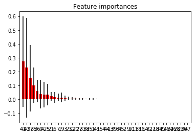
Ahhhhhh. Look at the top two features:
- collection_recovery_fee (0.254455)
- recoveries (0.219021)
The recovery fee recieved and the number of recoveries. These are directly related to loan defaults; you will only get a recovery if there is a loan default.
Clearly, we won’t have these features unless a default has already occured and in that case, there’s certainly no point in trying to predict it!
This is a perfect example of data leakage. This is where you use data that is impossible to obtain at the time, usually because it is a direct consequence of an event that you are trying to predict.
Just for further giggles, let’s plot a box plot of the recoveries data…
loan_amount = pd.DataFrame([selected["recoveries"], bad_indicator]).transpose()
loan_amount.boxplot(by="loan_status")
plt.show()
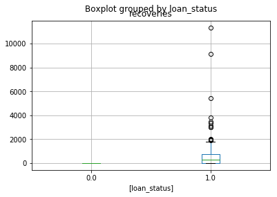
This is plotting the recoveries data by the loan status. Note how all of the “normal” loans have zero recoveries.
If this really was a feature we could just threshold above 0 and say it was “suffering”.
Hence why we got 95% in the accuracy score!
However, this begs the question, if this was so easy, why did we get 95% and not 100%?!?!
Let’s remove those features and try again…
X.drop(["collection_recovery_fee", "recoveries"], axis=1, inplace=True)
clf = RandomForestClassifier(max_depth=3)
clf = clf.fit(X, bad_indicator)
scores = cross_val_score(clf, X, bad_indicator, cv=5, scoring='accuracy')
print("Accuracy: %0.2f (+/- %0.2f)" % (scores.mean(), scores.std()))
Accuracy: 0.89 (+/- 0.01)
Ok, this is starting to look a bit more feasible
importances = clf.feature_importances_
std = np.std([tree.feature_importances_ for tree in clf.estimators_],
             axis=0)
indices = np.argsort(importances)[::-1]

# Print the feature ranking
print("Feature ranking:")

names = X.columns

for f in range(X.shape[1]):
    print("%d. %s (%f)" % (f + 1, names[indices[f]], importances[indices[f]]))

# Plot the feature importances of the forest
plt.figure()
plt.title("Feature importances")
plt.bar(range(X.shape[1]), importances[indices],
       color="r", yerr=std[indices], align="center")
plt.xticks(range(X.shape[1]), indices)
plt.xlim([-1, X.shape[1]])
# plt.savefig('../img/feature_importances.svg', transparent=True, bbox_inches='tight', pad_inches=0)
plt.show()
Feature ranking:
1. last_pymnt_amnt (0.168353)
2. total_rec_prncp (0.151796)
3. total_pymnt_inv (0.135874)
4. total_pymnt (0.069144)
5. funded_amnt (0.052595)
6. int_rate (0.049567)
7. revol_util (0.045033)
8. earliest_cr_line (0.044411)
9. out_prncp (0.039759)
10. total_rec_late_fee (0.037326)
11. last_credit_pull_d (0.032130)
12. sub_grade (0.026536)
13. revol_bal (0.021711)
14. dti (0.020970)
15. url (0.016244)
16. zip_code (0.013791)
17. grade (0.011085)
18. emp_length (0.009951)
19. purpose (0.008554)
20. verification_status (0.008065)
21. open_acc (0.007716)
22. emp_title (0.007045)
23. total_rec_int (0.006613)
24. total_acc (0.005885)
25. loan_amnt (0.005698)
26. addr_state (0.004147)
27. installment (0.000000)
28. issue_d (0.000000)
29. term (0.000000)
30. home_ownership (0.000000)
31. annual_inc (0.000000)
32. funded_amnt_inv (0.000000)
33. acc_now_delinq (0.000000)
34. pymnt_plan (0.000000)
35. desc (0.000000)
36. title (0.000000)
37. application_type (0.000000)
38. inq_last_6mths (0.000000)
39. mths_since_last_delinq (0.000000)
40. mths_since_last_record (0.000000)
41. pub_rec (0.000000)
42. initial_list_status (0.000000)
43. out_prncp_inv (0.000000)
44. collections_12_mths_ex_med (0.000000)
45. policy_code (0.000000)
46. delinq_2yrs (0.000000)
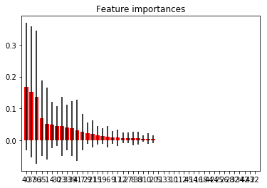
The best features now are:
- total_rec_prncp (0.232828)
- last_pymnt_amnt (0.145886)
- total_pymnt_inv (0.140592)
- total_pymnt (0.129989)
So it seems like there is some correlation with how much has been paid off and delinquincy.
We should look into these correlations more.
So, what we’d do now is chop off all except the first 10, maybe, and see if we can improve that data (with scaling, encoding, missing data imputing, etc.)
We would also consider mixtures of features, e.g. the proportion of the loan repaid, etc.