COVID-19 Logistic Bayesian Model
by Dr. Phil Winder , CEO
This post builds upon the exponential model created in a previous post. The main issue was that there an exponential model does not include a limit. A logistic model introduces this limit. I also perform some very basic backtesting and future prediction.
What is a Logistic Model?
The logistic model has an equation:
$$ \frac{dC}{dt} = rC\bigg(1 - \frac{C}{K}\bigg) $$
Where $C$ is an accumulated number of cases, $r > 0$ is the infection rate, and $K > 0$ is the final epidemic size. The solution of this equation is:
$$ C = \frac{K}{1 + Ae^{-rt}} $$
Where: $A = \frac{K - C_0}{C_0}$ and $C_0$ is the initial number of cases at time zero.
When I’m trying to understand a model, I find it useful to plot a few versions of the model with different parameters to find out how it behaves.
import numpy as np
import matplotlib.pyplot as plt
def C(K, r, t, C_0):
A = (K-C_0)/C_0
return K / (1 + A * np.exp(-r * t))
def d_C(K, r, t, C_0):
c = C(K, r, t, C_0)
return r * c * (1 - c / K)
r = 0.2
K = 1000
C_0 = 100
t = np.linspace(1,60)
fig, ax = plt.subplots(1, 2, figsize=(12,5))
for r in np.linspace(0.1, 0.5, 5):
ax[0].plot(t, C(K, r, t, C_0), label=f"r = {r:0.2f}")
ax[0].legend(loc="best")
ax[0].set(xlabel="Days since...", ylabel="Cases")
for K in np.linspace(100, 10000, 10):
ax[1].plot(t, C(K, r, t, C_0), label=f"K = {K:0.1f}")
ax[1].legend(loc="best")
ax[1].set(xlabel="Days since...", ylabel="Cases")
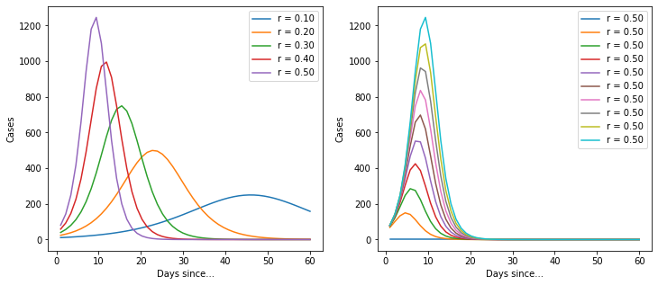
fig, ax = plt.subplots(1, 2, figsize=(12,5))
for r in np.linspace(0.1, 0.5, 5):
ax[0].plot(t, d_C(K, r, t, C_0), label=f"r = {r:0.2f}")
ax[0].legend(loc="best")
ax[0].set(xlabel="Days since...", ylabel="Cases")
for K in np.linspace(100, 10000, 10):
ax[1].plot(t, d_C(K, r, t, C_0), label=f"r = {r:0.2f}")
ax[1].legend(loc="best")
ax[1].set(xlabel="Days since...", ylabel="Cases")
[Text(0, 0.5, 'Cases'), Text(0.5, 0, 'Days since...')]
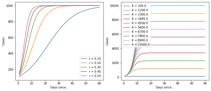
Ok, so it’s a basic logistic function. But it’s quite useful because it implicitly provides an estimate for the total number of cases. Let’s import the data again and build a model.
Initialisation and Imports
!pip install arviz pymc3==3.8
import numpy as np
import pymc3 as pm
import pandas as pd
import matplotlib.pyplot as plt
import theano

# Load data
df = pd.read_csv("https://opendata.ecdc.europa.eu/covid19/casedistribution/csv/", parse_dates=["dateRep"], infer_datetime_format=True, dayfirst=True)
df = df.rename(columns={'dateRep': 'date', 'countriesAndTerritories': 'country'}) # Sane column names
df = df.drop(["day", "month", "year", "geoId"], axis=1) # Not required

country = "China"
# Filter for country (probably want separate models per country, even maybe per region)
sorted_country = df[df["country"] == country].sort_values(by="date")
# Cumulative sum of data
country_cumsum = sorted_country[["cases", "deaths"]].cumsum().set_index(sorted_country["date"])
# Filter out data with less than 100 cases
country_cumsum = country_cumsum[country_cumsum["cases"] >= 100]
days_since_100 = range(len(country_cumsum))

# Pull out population size per country
populations = {key: df[df["country"] == key].iloc[0]["popData2018"] for key in df["country"].unique()}
Logistic Model
def model_factory(country: str, x: np.ndarray, y: np.ndarray):
  with pm.Model() as model:
    t = pm.Data(country + "x_data", x)
    confirmed_cases = pm.Data(country + "y_data", y)

    # Intercept - We fixed this at 100.
    C_0 = pm.Normal("C_0", mu=100, sigma=10)

    # Growth rate: 0.2 is approx value reported by others
    r = pm.Normal("r", mu=0.2, sigma=0.5)

    # Total number of cases. Depends on the population, more people, more infections.
    # It also depends on the total number of people infected.
    # Start with a prior based upon a guess of the initial population, very weak
    proportion_infected = 5e-05 # This value comes from the rough projection that 80000 will be infected in China
    p = populations[country]
    K = pm.Normal("K", mu=p * proportion_infected, sigma=p*0.1)

    # Logistic regression
    growth = C(K, r, t, C_0)

    # Likelihood error
    eps = pm.HalfNormal("eps")

    # Likelihood - Counts here, so poission or negative binomial. Causes issues. Lognormal tends to work better?
    pm.Lognormal(country, mu=np.log(growth), sigma=eps, observed=confirmed_cases)
  return model
Model Testing
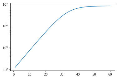
Let’s train it on some synthetic data to begin with to make sure the model can actually fit it. Someone more experienced wouldn’t need to do this!
r = 0.2
K = 80000 # This should look something a bit like China
C_0 = 100
t = np.linspace(1,60)
y_synthetic = C(K, r, t, C_0)
plt.plot(t, y_synthetic)
plt.gca().set_yscale("log")
# Training
with model_factory(country, t, y_synthetic) as model:
train_trace = pm.sample()
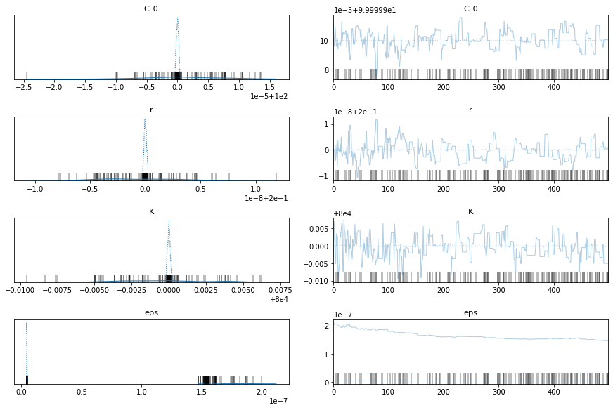
pm.traceplot(train_trace)
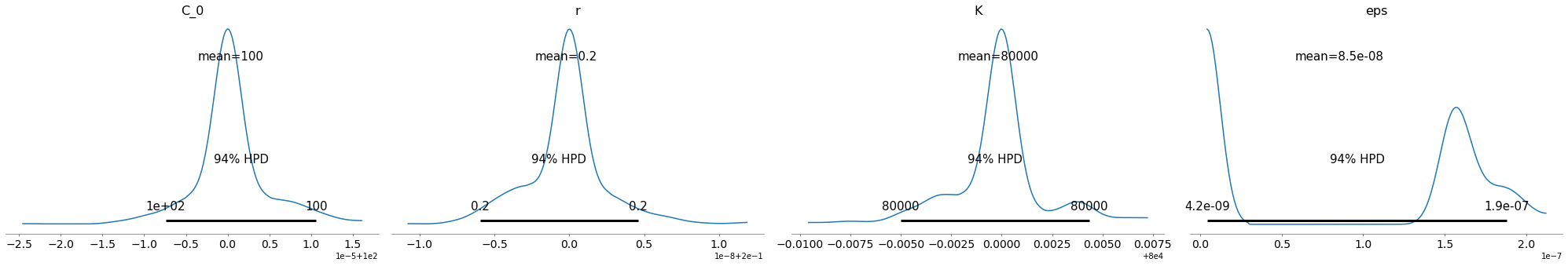
pm.plot_posterior(train_trace)
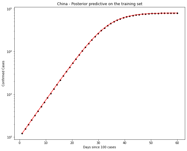
ppc = pm.sample_posterior_predictive(train_trace)
fig, ax = plt.subplots(figsize=(10, 8))
ax.plot(t, ppc[country].T, ".k", alpha=0.05)
ax.plot(t, y_synthetic, color="r")
ax.set_yscale("log")
ax.set(xlabel="Days since 100 cases", ylabel="Confirmed Cases", title=f"{country} - Posterior predictive on the training set")
Auto-assigning NUTS sampler...
Initializing NUTS using jitter+adapt_diag...
Sequential sampling (2 chains in 1 job)
NUTS: [eps, K, r, C_0]
Sampling chain 0, 89 divergences: 100%|██████████| 1000/1000 [00:06<00:00, 149.55it/s]
Sampling chain 1, 62 divergences: 100%|██████████| 1000/1000 [00:11<00:00, 90.78it/s]
There were 89 divergences after tuning. Increase `target_accept` or reparameterize.
The acceptance probability does not match the target. It is 0.18427594891059368, but should be close to 0.8. Try to increase the number of tuning steps.
There were 151 divergences after tuning. Increase `target_accept` or reparameterize.
The acceptance probability does not match the target. It is 0.2022248971431065, but should be close to 0.8. Try to increase the number of tuning steps.
The rhat statistic is larger than 1.4 for some parameters. The sampler did not converge.
The estimated number of effective samples is smaller than 200 for some parameters.
100%|██████████| 1000/1000 [00:10<00:00, 92.99it/s]
China Data
Ok, the above seems to work ok. The K parameter is quite important here. There are a distinct lack of confirmed cases relative to the population.
Let’s give it a whirl on real data.
train_x = days_since_100[:-5]
train_y = country_cumsum["cases"].astype('float64').values[:-5]
hold_out_x = days_since_100[-5:]
hold_out_y = country_cumsum["cases"].astype('float64').values[-5:]
# Training
with model_factory(country, train_x, train_y) as model:
    train_trace = pm.sample()
    pm.traceplot(train_trace)
    pm.plot_posterior(train_trace)
    ppc = pm.sample_posterior_predictive(train_trace)
    fig, ax = plt.subplots(figsize=(10, 8))
    ax.plot(train_x, ppc[country].T, ".k", alpha=0.05)
    ax.plot(train_x, train_y, color="r")
    ax.set_yscale("log")
    ax.set(xlabel="Date", ylabel="Confirmed Cases", title=f"{country} - Posterior predictive on the training set")
Auto-assigning NUTS sampler...
Initializing NUTS using jitter+adapt_diag...
Sequential sampling (2 chains in 1 job)
NUTS: [eps, K, r, C_0]
Sampling chain 0, 0 divergences: 100%|██████████| 1000/1000 [00:03<00:00, 295.79it/s]
Sampling chain 1, 0 divergences: 100%|██████████| 1000/1000 [00:01<00:00, 838.63it/s]
100%|██████████| 1000/1000 [00:10<00:00, 98.26it/s]
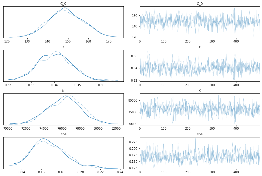
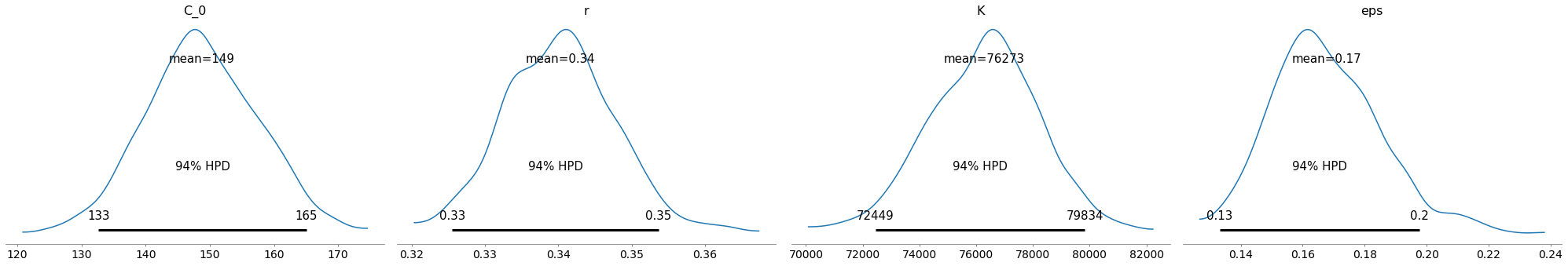
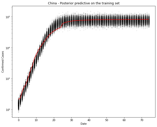
Yep, that looks ok. Let’s test. I can’t imagine it will be too wrong, since it’s practically a straight line now.
# New model with holdout data
with model_factory(country, hold_out_x, hold_out_y) as test_model:
ppc = pm.sample_posterior_predictive(train_trace)
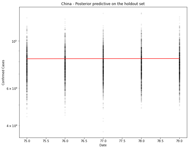
fig, ax = plt.subplots(figsize=(10, 8))
ax.plot(hold_out_x, ppc[country].T, ".k", alpha=0.05)
ax.plot(hold_out_x, hold_out_y, color="r")
ax.set_yscale("log")
ax.set(xlabel="Date", ylabel="Confirmed Cases", title=f"{country} - Posterior predictive on the holdout set")
100%|██████████| 1000/1000 [00:10<00:00, 93.52it/s]
# Generate the predicted number of cases (assuming normally distributed on the output)
predicted_cases = ppc[country].mean(axis=0).round()
print(predicted_cases)
def error(actual, predicted):
  return predicted - actual

def print_errors(actuals, predictions):
  for n in [1, 5]:
    act, pred = actuals[n-1], predictions[n-1]
    err = error(act, pred)
    print(f"{n}-day cumulative prediction error: {err} cases ({100 * err / act:.1f} %)")

print_errors(hold_out_y, predicted_cases)
[76862. 77142. 77070. 77337. 77369.]
1-day cumulative prediction error: -5603.0 cases (-6.8 %)
5-day cumulative prediction error: -5329.0 cases (-6.4 %)
new_x = [hold_out_x[-1] + 1, hold_out_x[-1] + 5]
new_y = [0, 0]
# Predictive model
with model_factory(country, new_x, new_y) as test_model:
    ppc = pm.sample_posterior_predictive(train_trace)
predicted_cases = ppc[country].mean(axis=0).round()
print("\n")
print(f"Based upon this model, tomorrow's number of cases will be {predicted_cases[0]}. In 5 days time there will be {predicted_cases[1]} cases.")
100%|██████████| 1000/1000 [00:10<00:00, 91.94it/s]


Based upon this model, tomorrow's number of cases will be 76879.0. In 5 days time there will be 78040.0 cases.
NOTE: These numbers are based upon a bad model. Don't use them!
UK Data
Let’s try that again with UK data.
country = "United_Kingdom"
# Filter for country (probably want separate models per country, even maybe per region)
sorted_country = df[df["country"] == country].sort_values(by="date")
# Cumulative sum of data
country_cumsum = sorted_country[["cases", "deaths"]].cumsum().set_index(sorted_country["date"])
# Filter out data with less than 100 cases
country_cumsum = country_cumsum[country_cumsum["cases"] >= 100]
days_since_100 = range(len(country_cumsum))

# Pull out population size per country
populations = {key: df[df["country"] == key].iloc[0]["popData2018"] for key in df["country"].unique()}
train_x = days_since_100[:-5]
train_y = country_cumsum["cases"].astype('float64').values[:-5]
hold_out_x = days_since_100[-5:]
hold_out_y = country_cumsum["cases"].astype('float64').values[-5:]
# Training
with model_factory(country, train_x, train_y) as model:
    train_trace = pm.sample()
    pm.traceplot(train_trace)
    pm.plot_posterior(train_trace)
    ppc = pm.sample_posterior_predictive(train_trace)
    fig, ax = plt.subplots(figsize=(10, 8))
    ax.plot(train_x, ppc[country].T, ".k", alpha=0.05)
    ax.plot(train_x, train_y, color="r")
    ax.set_yscale("log")
    ax.set(xlabel="Date", ylabel="Confirmed Cases", title=f"{country} - Posterior predictive on the training set")
Auto-assigning NUTS sampler...
Initializing NUTS using jitter+adapt_diag...
Sequential sampling (2 chains in 1 job)
NUTS: [eps, K, r, C_0]
Sampling chain 0, 0 divergences: 100%|██████████| 1000/1000 [00:03<00:00, 262.76it/s]
Sampling chain 1, 0 divergences: 100%|██████████| 1000/1000 [00:03<00:00, 311.88it/s]
The acceptance probability does not match the target. It is 0.901537203821684, but should be close to 0.8. Try to increase the number of tuning steps.
100%|██████████| 1000/1000 [00:10<00:00, 93.39it/s]
Yep, that looks ok. Let’s test. I can’t imagine it will be too wrong, since it’s practically a straight line now.
# New model with holdout data
with model_factory(country, hold_out_x, hold_out_y) as test_model:
ppc = pm.sample_posterior_predictive(train_trace)
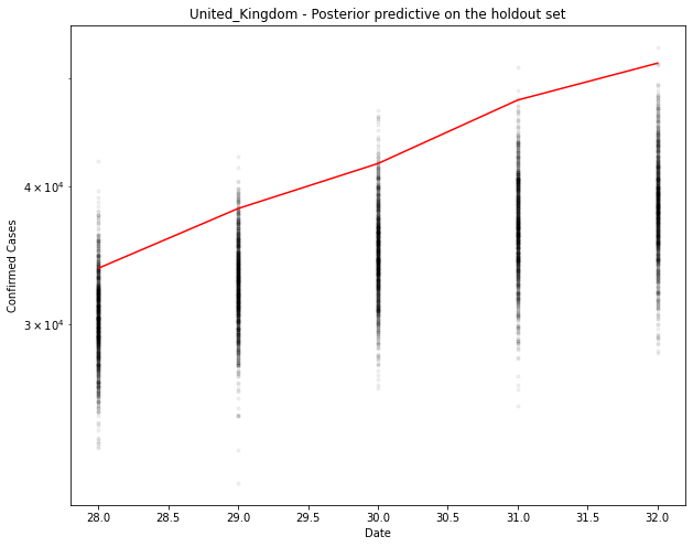
fig, ax = plt.subplots(figsize=(10, 8))
ax.plot(hold_out_x, ppc[country].T, ".k", alpha=0.05)
ax.plot(hold_out_x, hold_out_y, color="r")
ax.set_yscale("log")
ax.set(xlabel="Date", ylabel="Confirmed Cases", title=f"{country} - Posterior predictive on the holdout set")
100%|██████████| 1000/1000 [00:10<00:00, 92.85it/s]
# Generate the predicted number of cases (assuming normally distributed on the output)
predicted_cases = ppc[country].mean(axis=0).round()
print(predicted_cases)
def error(actual, predicted):
  return predicted - actual

def print_errors(actuals, predictions):
  for n in [1, 5]:
    act, pred = actuals[n-1], predictions[n-1]
    err = error(act, pred)
    print(f"{n}-day cumulative prediction error: {err} cases ({100 * err / act:.1f} %)")

print_errors(hold_out_y, predicted_cases)
[30386. 32655. 34929. 36882. 38485.]
1-day cumulative prediction error: -3332.0 cases (-9.9 %)
5-day cumulative prediction error: -13123.0 cases (-25.4 %)
new_x = [hold_out_x[-1] + 1, hold_out_x[-1] + 5]
new_y = [0, 0]
# Predictive model
with model_factory(country, new_x, new_y) as test_model:
    ppc = pm.sample_posterior_predictive(train_trace)
predicted_cases = ppc[country].mean(axis=0).round()
print("\n")
print(f"Based upon this model, tomorrow's number of cases will be {predicted_cases[0]}. In 5 days time there will be {predicted_cases[1]} cases.")
100%|██████████| 1000/1000 [00:10<00:00, 92.23it/s]


Based upon this model, tomorrow's number of cases will be 40037.0. In 5 days time there will be 43740.0 cases.
Slightly under for the UK. It seems to be tailing off a bit before the model predicts it should.