COVID-19 Hierarchical Bayesian Logistic Model with pymc3
by Dr. Phil Winder , CEO
I have two outstanding tasks from the previous notebooks. The first is that I haven’t iterated over all countries.
The task relates to how we constrain the parameters of each country. It makes sense to use the global average to constrain the other estimates. For example, if we assume this is the same virus and has the same parameters no matter where it is (the same transmission rate, for example) then we should be able to estimate high level parameters and derive country level specifics (it transmits better in warm countries, for example). You can achieve this in Bayesian modeling through hierarchical models.
There is a lot of code in this notebook and that is intentional. I wanted to try and demonstrate the number of iterations required to improve a model. And I’m not even trying to improve the underlying model, just the way in which a logistic fits the data.
If you are interested in the final result, then skip to the bottom.
First let me reload/import all the stuff from the previous notebook.
!pip install arviz pymc3==3.8
import numpy as np
import pymc3 as pm
import pandas as pd
import matplotlib.pyplot as plt
import theano

def logistic(K, r, t, C_0):
  A = (K-C_0)/C_0
  return K / (1 + A * np.exp(-r * t))

# Load data
df = pd.read_csv("https://opendata.ecdc.europa.eu/covid19/casedistribution/csv/", parse_dates=["dateRep"], infer_datetime_format=True, dayfirst=True)
df = df.rename(columns={'dateRep': 'date', 'countriesAndTerritories': 'country'}) # Sane column names
df = df.drop(["day", "month", "year", "geoId"], axis=1) # Not required

# Create DF with sorted index
sorted_data = df.set_index(df["date"]).sort_index()
sorted_data["cumulative_cases"] = sorted_data.groupby(by="country")["cases"].cumsum()
sorted_data["cumulative_deaths"] = sorted_data.groupby(by="country")["cases"].cumsum()

# Filter out data with less than 500 cases, we probably can't get very good estimates from these.
sorted_data = sorted_data[sorted_data["cumulative_cases"] >= 500]

# Remove "Czechia" it has a population of NaN
sorted_data = sorted_data[sorted_data["country"] != "Czechia"]

# Get final list of countries
countries = sorted_data["country"].unique()
n_countries = len(countries)

# Pull out population size per country
populations = {country: df[df["country"] == country].iloc[0]["popData2018"] for country in countries}

# A map from country to integer index (for the model)
idx_country = pd.Index(countries).get_indexer(sorted_data.country)

# Create a new column with the number of days since first infection (the x-axis)
country_first_dates = {c: sorted_data[sorted_data["country"] == c].index.min() for c in countries}
sorted_data["100_cases"] = sorted_data.apply(lambda x: country_first_dates[x.country], axis=1)
sorted_data["days_since_100_cases"] = (sorted_data.index - sorted_data["100_cases"]).apply(lambda x: x.days)
Pooled Model
Now I want to rebuild the model to generate estimates for every country in the dataset.
This step is much more tricky that it first seems. First, if you don’t remove the small number of cases, then it continuously produces nans because initially the estimates are sub-zero and the log doesn’t like it. So that’s why we need days_since_100_cases.
Next, passing all the data into the model is tricky. You could do a big for loop, but it takes forrr eeeever. So instead, you have to vectorise your code and it can be difficult to get right.
Also remember that this is a logistic shape - an S shape - so the data needs to be a cumulative sum. I forgot that and I couldn’t figure out why I was getting bad energy messages from pymc3. Turned out the data fit too poorly.
Another tip. When you are building a model based upon data that has multiple sources, build a model for each parameter individually, to test that the model is stable. I found several times that one of my parameters in my model was blowing up everything else. Strip everything back and test one thing at a time.
For example, begin by creating one massive pooled model. If this doesn’t work, then individual models won’t work. Next, try building in individual models but only for a single parameter. Go through each, one by one. If they all work, then try them in combination.
But first, I need a baseline. The baseline is the “pooled” model, or in other words, the model that uses the same parameters for all countries.
pooled_model = pm.Model("Pooled")
with pooled_model:
    BoundedNormal = pm.Bound(pm.Normal, lower=0.0)
    t = pm.Data("x_data", sorted_data["days_since_100_cases"])
    confirmed_cases = pm.Data("y_data", sorted_data["cumulative_cases"])

    # Intercept - We fixed this at 100.
    C_0 = pm.Normal("C_0", mu=100, sigma=10)

    # Growth rate: 0.2 is approx value reported by others
    r = BoundedNormal("r", mu=0.2, sigma=0.1)

    # Total number of cases. Depends on the population, more people, more infections.
    proportion_infected = 5e-05 # This value comes from the rough projection that 80000 will be infected in China
    p = sorted_data.popData2018.mean() # Crude. Can have a mean per country. Not sure how to do this
    K = pm.Normal("K", mu=p * proportion_infected, sigma=p*0.1)#, shape=n_countries)

    # Logistic regression
    growth = logistic(K, r, t, C_0)

    # Likelihood error
    eps = pm.HalfNormal("eps")

    # Likelihood - Counts here, so poission or negative binomial. Causes issues. Lognormal tends to work better?
    pm.Lognormal("cases", mu=np.log(growth), sigma=eps, observed=confirmed_cases)

pm.model_to_graphviz(pooled_model)

The code below is a very handy function that I found on the pymc3 forum somewhere. It picks a random test point and samples the posterior. If the result produces nan then you know you have a problem. The sampling will fail if that is the case.
# Test that the model does not produce NaNs. If it does, it can't converge.
for RV in pooled_model.basic_RVs:
    print(RV.name, RV.logp(pooled_model.test_point))
Pooled_C_0 -3.2215236261987186
Pooled_r_lowerbound__ -30.616353440210627
Pooled_K -17.26574353862072
Pooled_eps_log__ -0.7698925914732455
Pooled_cases -18218.268119660002
with pooled_model:
  pooled_trace = pm.sample()
Auto-assigning NUTS sampler...
Initializing NUTS using jitter+adapt_diag...
Sequential sampling (2 chains in 1 job)
NUTS: [Pooled_eps, Pooled_K, Pooled_r, Pooled_C_0]
Sampling chain 0, 0 divergences: 100%|██████████| 1000/1000 [00:05<00:00, 184.21it/s]
Sampling chain 1, 0 divergences: 100%|██████████| 1000/1000 [00:05<00:00, 197.76it/s]
The acceptance probability does not match the target. It is 0.8911189225404523, but should be close to 0.8. Try to increase the number of tuning steps.
pm.traceplot(pooled_trace);
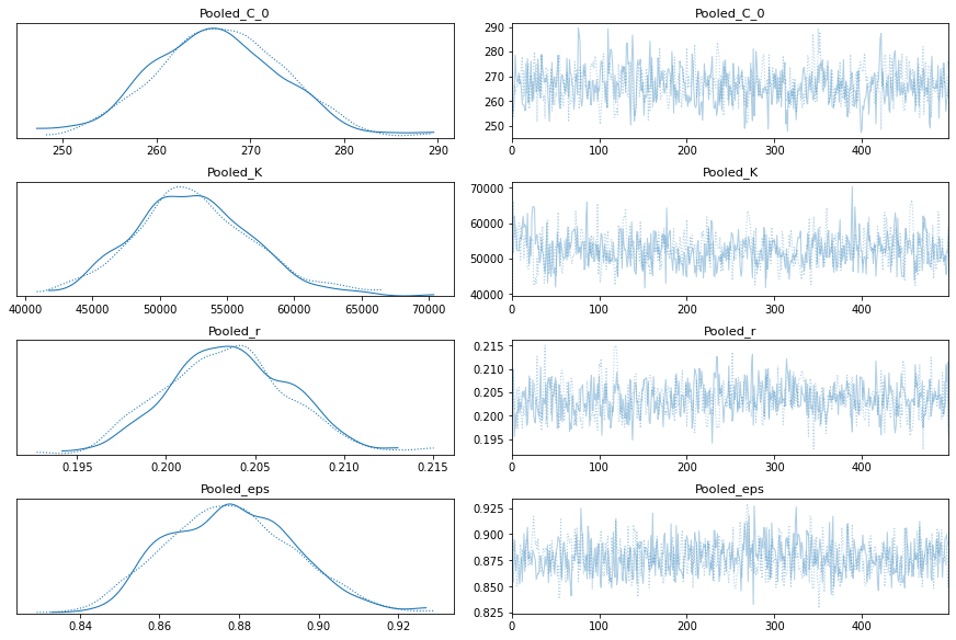
Model With Total Cases per Country
Now let me build a model with a country-specific value for K.
total_per_country_model = pm.Model("Total per country")
with total_per_country_model:
    BoundedNormal = pm.Bound(pm.Normal, lower=0.0)
    t = pm.Data("x_data", sorted_data["days_since_100_cases"])
    confirmed_cases = pm.Data("y_data", sorted_data["cumulative_cases"])

    # Intercept - We fixed this at 100.
    C_0 = pm.Normal("C_0", mu=100, sigma=10)

    # Growth rate: 0.2 is approx value reported by others
    r = BoundedNormal("r", mu=0.2, sigma=0.1)

    # Total number of cases. Depends on the population, more people, more infections.
    proportion_infected = 5e-05 # This value comes from the rough projection that 80000 will be infected in China
    p = sorted_data.popData2018.mean() # Crude. Can have a mean per country. Not sure how to do this
    K = pm.Normal("K", mu=p * proportion_infected, sigma=p*0.1, shape=n_countries)

    # Logistic regression
    growth = logistic(K[idx_country], r, t, C_0)

    # Likelihood error
    eps = pm.HalfNormal("eps")

    # Likelihood - Counts here, so poission or negative binomial. Causes issues. Lognormal tends to work better?
    pm.Lognormal("cases", mu=np.log(growth), sigma=eps, observed=confirmed_cases)

pm.model_to_graphviz(total_per_country_model)

with total_per_country_model:
  total_per_country_trace = pm.sample()
Auto-assigning NUTS sampler...
Initializing NUTS using jitter+adapt_diag...
Sequential sampling (2 chains in 1 job)
NUTS: [Total per country_eps, Total per country_K, Total per country_r, Total per country_C_0]
Sampling chain 0, 143 divergences: 100%|██████████| 1000/1000 [04:39<00:00,  3.58it/s]
Sampling chain 1, 126 divergences: 100%|██████████| 1000/1000 [05:40<00:00,  2.93it/s]
There were 143 divergences after tuning. Increase `target_accept` or reparameterize.
The chain reached the maximum tree depth. Increase max_treedepth, increase target_accept or reparameterize.
There were 269 divergences after tuning. Increase `target_accept` or reparameterize.
The chain reached the maximum tree depth. Increase max_treedepth, increase target_accept or reparameterize.
The rhat statistic is larger than 1.05 for some parameters. This indicates slight problems during sampling.
The estimated number of effective samples is smaller than 200 for some parameters.
pm.traceplot(total_per_country_trace);
pm.forestplot(total_per_country_trace, var_names=['Total per country_K']);
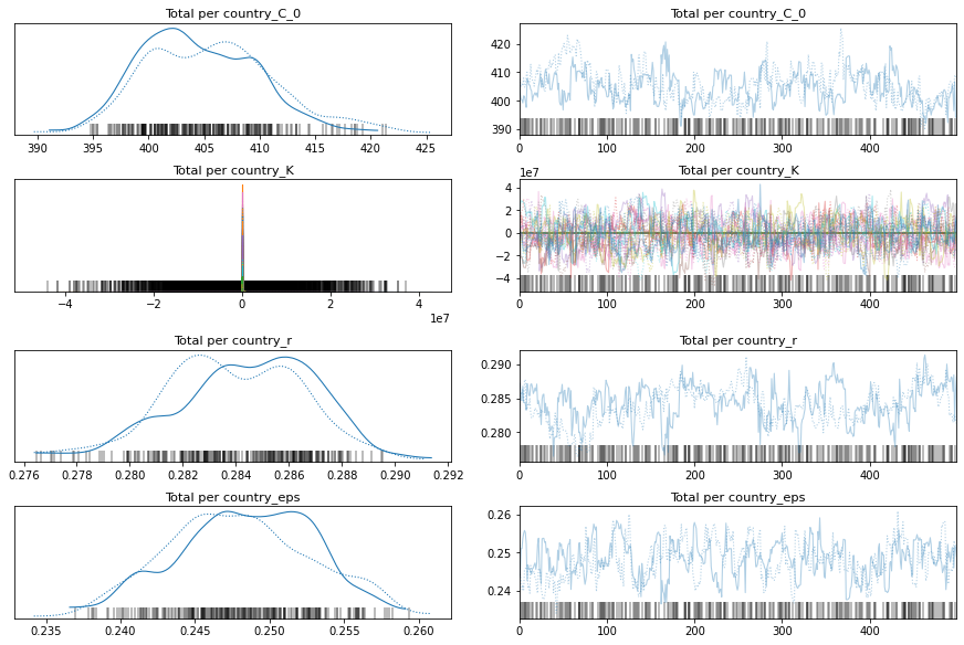
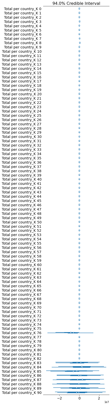
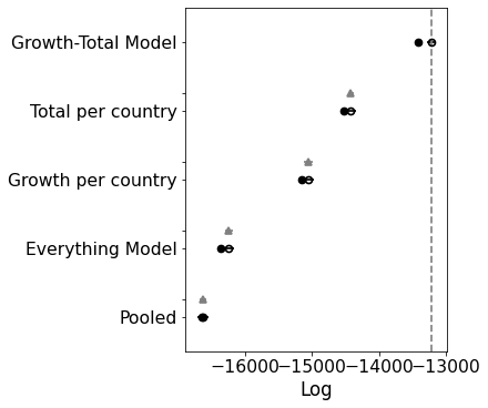
Comparison Between Pooled and K per Country Model
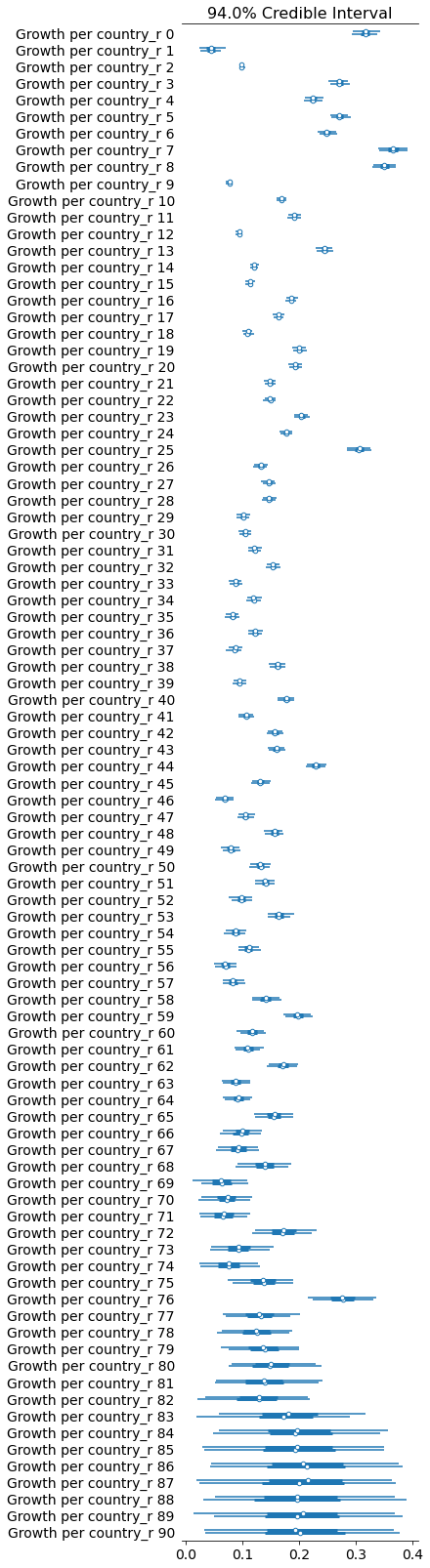
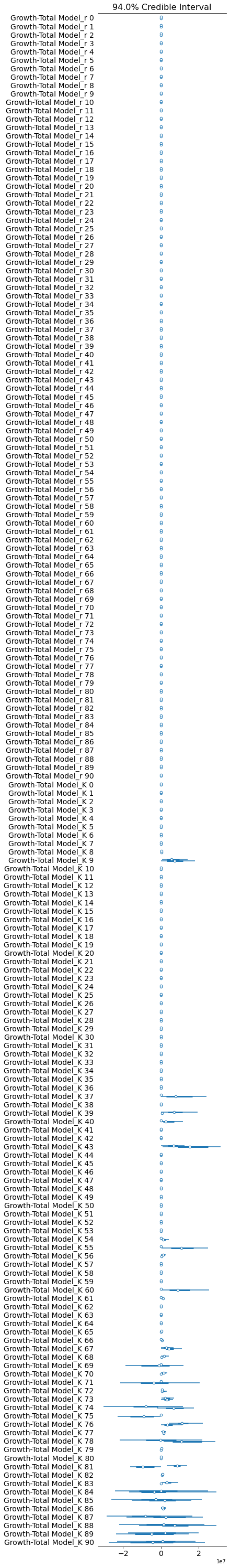
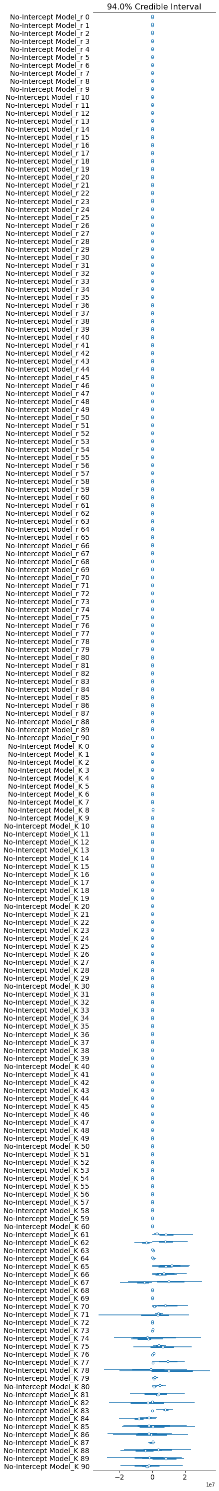
If you look at the traces above, you can see that some of the countries (near the bottom) have an wildly uncertain estimate for K. The lower countries, because of the way the data is sorted, are countries that don’t have many cases.
We could remove those countries, but let’s leave them in for now.
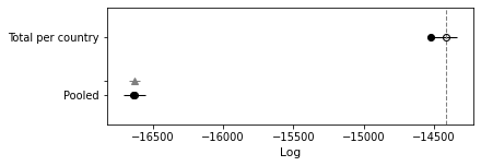
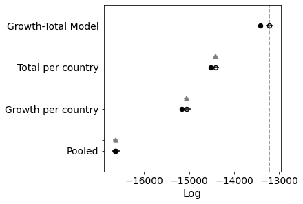
Below I use leave one out cross validation, where the algorithm iteratively removes observations and compares the prediction. Higher values are better.
You can see that the K-per-country model is significantly better.
comparison = pm.compare({pooled_model.name: pooled_trace, total_per_country_model.name: total_per_country_trace}, ic='LOO')
print(comparison)
pm.compareplot(comparison);
                  rank      loo    p_loo  ...     dse warning loo_scale
Total per country    0 -14416.5  52.1214  ...       0   False       log
Pooled               1 -16629.8  4.14689  ...  39.679   False       log

[2 rows x 9 columns]
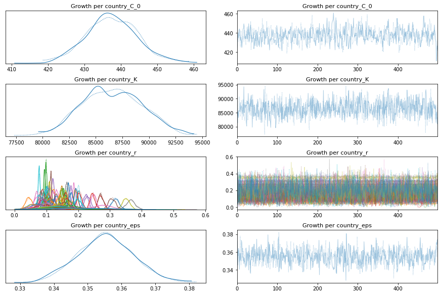
Model with per-country growth rates
Ok, so now let’s build a model with per-country growth rates.
growth_per_country_model = pm.Model("Growth per country")
with growth_per_country_model:
    BoundedNormal = pm.Bound(pm.Normal, lower=0.0)
    t = pm.Data("x_data", sorted_data["days_since_100_cases"])
    confirmed_cases = pm.Data("y_data", sorted_data["cumulative_cases"])

    # Intercept - We fixed this at 100.
    C_0 = pm.Normal("C_0", mu=100, sigma=10)

    # Growth rate: 0.2 is approx value reported by others
    r = BoundedNormal("r", mu=0.2, sigma=0.1, shape=n_countries)

    # Total number of cases. Depends on the population, more people, more infections.
    proportion_infected = 5e-05 # This value comes from the rough projection that 80000 will be infected in China
    p = sorted_data.popData2018.mean() # Crude. Can have a mean per country. Not sure how to do this
    K = pm.Normal("K", mu=p * proportion_infected, sigma=p*0.1)

    # Logistic regression
    growth = logistic(K, r[idx_country], t, C_0)

    # Likelihood error
    eps = pm.HalfNormal("eps")

    # Likelihood - Counts here, so poission or negative binomial. Causes issues. Lognormal tends to work better?
    pm.Lognormal("cases", mu=np.log(growth), sigma=eps, observed=confirmed_cases)

pm.model_to_graphviz(growth_per_country_model)

with growth_per_country_model:
  growth_per_country_trace = pm.sample()
pm.traceplot(growth_per_country_trace);
pm.forestplot(growth_per_country_trace, var_names=['Growth per country_r']);
Auto-assigning NUTS sampler...
Initializing NUTS using jitter+adapt_diag...
Sequential sampling (2 chains in 1 job)
NUTS: [Growth per country_eps, Growth per country_K, Growth per country_r, Growth per country_C_0]
Sampling chain 0, 0 divergences: 100%|██████████| 1000/1000 [00:11<00:00, 84.38it/s]
Sampling chain 1, 0 divergences: 100%|██████████| 1000/1000 [00:11<00:00, 85.54it/s]
The acceptance probability does not match the target. It is 0.9001435860072379, but should be close to 0.8. Try to increase the number of tuning steps.
comparison = pm.compare({pooled_model.name: pooled_trace, total_per_country_model.name: total_per_country_trace, growth_per_country_model.name: growth_per_country_trace}, ic='LOO')
print(comparison)
pm.compareplot(comparison);
/usr/local/lib/python3.6/dist-packages/arviz/stats/stats.py:532: UserWarning: Estimated shape parameter of Pareto distribution is greater than 0.7 for one or more samples. You should consider using a more robust model, this is because importance sampling is less likely to work well if the marginal posterior and LOO posterior are very different. This is more likely to happen with a non-robust model and highly influential observations.
  "Estimated shape parameter of Pareto distribution is greater than 0.7 for "

                   rank      loo    p_loo  ...      dse warning loo_scale
Total per country     0 -14416.5  52.1214  ...        0   False       log
Growth per country    1 -15052.1  54.3001  ...  60.7668    True       log
Pooled                2 -16629.8  4.14689  ...   39.679   False       log

[3 rows x 9 columns]
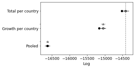
Comparing again you can see that it has improved the model as well, although not quite as much as the other. Let’s try and combine them.
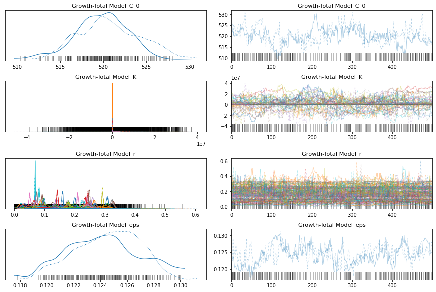
Per-Country Growth and Total Model
growth_total_model = pm.Model("Growth-Total Model")
with growth_total_model:
    BoundedNormal = pm.Bound(pm.Normal, lower=0.0)
    t = pm.Data("x_data", sorted_data["days_since_100_cases"])
    confirmed_cases = pm.Data("y_data", sorted_data["cumulative_cases"])

    # Intercept - We fixed this at 100.
    C_0 = pm.Normal("C_0", mu=100, sigma=10)

    # Growth rate: 0.2 is approx value reported by others
    r = BoundedNormal("r", mu=0.2, sigma=0.1, shape=n_countries)

    # Total number of cases. Depends on the population, more people, more infections.
    proportion_infected = 5e-05 # This value comes from the rough projection that 80000 will be infected in China
    p = sorted_data.popData2018.mean() # Crude. Can have a mean per country. Not sure how to do this
    K = pm.Normal("K", mu=p * proportion_infected, sigma=p*0.1, shape=n_countries)

    # Logistic regression
    growth = logistic(K[idx_country], r[idx_country], t, C_0)

    # Likelihood error
    eps = pm.HalfNormal("eps")

    # Likelihood - Counts here, so poission or negative binomial. Causes issues. Lognormal tends to work better?
    pm.Lognormal("cases", mu=np.log(growth), sigma=eps, observed=confirmed_cases)

pm.model_to_graphviz(growth_total_model)

with growth_total_model:
  growth_total_trace = pm.sample()
pm.traceplot(growth_total_trace);
pm.forestplot(growth_total_trace, var_names=['Growth-Total Model_r', 'Growth-Total Model_K']);
Auto-assigning NUTS sampler...
Initializing NUTS using jitter+adapt_diag...
Sequential sampling (2 chains in 1 job)
NUTS: [Growth-Total Model_eps, Growth-Total Model_K, Growth-Total Model_r, Growth-Total Model_C_0]
Sampling chain 0, 123 divergences: 100%|██████████| 1000/1000 [05:50<00:00,  2.85it/s]
Sampling chain 1, 75 divergences: 100%|██████████| 1000/1000 [06:13<00:00,  2.68it/s]
There were 123 divergences after tuning. Increase `target_accept` or reparameterize.
The chain reached the maximum tree depth. Increase max_treedepth, increase target_accept or reparameterize.
There were 198 divergences after tuning. Increase `target_accept` or reparameterize.
The chain reached the maximum tree depth. Increase max_treedepth, increase target_accept or reparameterize.
The rhat statistic is larger than 1.4 for some parameters. The sampler did not converge.
The estimated number of effective samples is smaller than 200 for some parameters.
comparison = pm.compare(
    {
      pooled_model.name: pooled_trace,
      total_per_country_model.name: total_per_country_trace,
      growth_per_country_model.name: growth_per_country_trace,
      growth_total_model.name: growth_total_trace
    }, ic='LOO');
print(comparison)
pm.compareplot(comparison);
/usr/local/lib/python3.6/dist-packages/arviz/stats/stats.py:532: UserWarning: Estimated shape parameter of Pareto distribution is greater than 0.7 for one or more samples. You should consider using a more robust model, this is because importance sampling is less likely to work well if the marginal posterior and LOO posterior are very different. This is more likely to happen with a non-robust model and highly influential observations.
  "Estimated shape parameter of Pareto distribution is greater than 0.7 for "

                   rank      loo    p_loo  ...      dse warning loo_scale
Growth-Total Model    0 -13219.6  98.6516  ...        0    True       log
Total per country     1 -14416.5  52.1214  ...  44.5365   False       log
Growth per country    2 -15052.1  54.3001  ...  66.2718    True       log
Pooled                3 -16629.8  4.14689  ...   56.487   False       log

[4 rows x 9 columns]
Great! Better again.
Everything per-country
The last thing to parameterise is the intercept. I’m not convinced that there will be much improvement here, because all of them were clipped at 100 cases. But let’s try.
everything_model = pm.Model("Everything Model")
with everything_model:
    BoundedNormal = pm.Bound(pm.Normal, lower=0.0)
    t = pm.Data("x_data", sorted_data["days_since_100_cases"])
    confirmed_cases = pm.Data("y_data", sorted_data["cumulative_cases"])

    # Intercept - We fixed this at 100.
    C_0 = pm.Normal("C_0", mu=100, sigma=10, shape=n_countries)

    # Growth rate: 0.2 is approx value reported by others
    r = BoundedNormal("r", mu=0.2, sigma=0.1, shape=n_countries)

    # Total number of cases. Depends on the population, more people, more infections.
    proportion_infected = 5e-05 # This value comes from the rough projection that 80000 will be infected in China
    p = sorted_data.popData2018.mean() # Crude. Can have a mean per country. Not sure how to do this
    K = pm.Normal("K", mu=p * proportion_infected, sigma=p*0.1, shape=n_countries)

    # Logistic regression
    growth = logistic(K[idx_country], r[idx_country], t, C_0[idx_country])

    # Likelihood error
    eps = pm.HalfNormal("eps")

    # Likelihood - Counts here, so poission or negative binomial. Causes issues. Lognormal tends to work better?
    pm.Lognormal("cases", mu=np.log(growth), sigma=eps, observed=confirmed_cases)

pm.model_to_graphviz(everything_model)

with everything_model:
everything_trace = pm.sample()
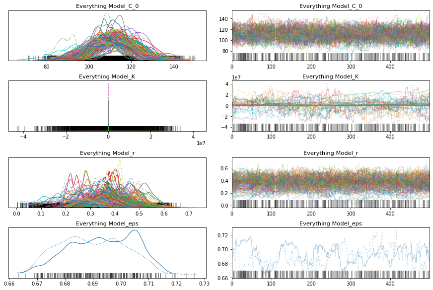
pm.traceplot(everything_trace);
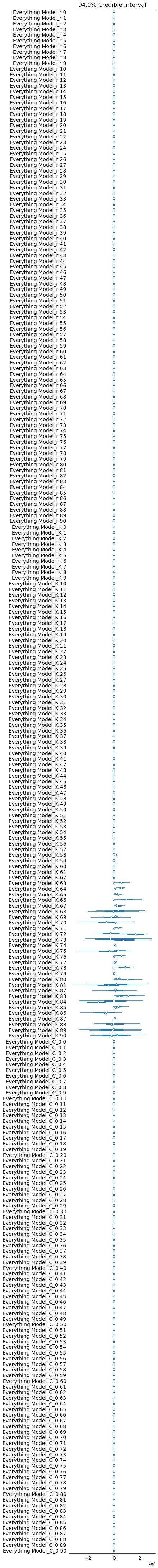
pm.forestplot(everything_trace, var_names=['Everything Model_r', 'Everything Model_K', 'Everything Model_C_0']);
Auto-assigning NUTS sampler...
Initializing NUTS using jitter+adapt_diag...
Sequential sampling (2 chains in 1 job)
NUTS: [Everything Model_eps, Everything Model_K, Everything Model_r, Everything Model_C_0]
Sampling chain 0, 110 divergences: 100%|██████████| 1000/1000 [06:08<00:00,  2.71it/s]
Sampling chain 1, 127 divergences: 100%|██████████| 1000/1000 [05:57<00:00,  2.80it/s]
There were 110 divergences after tuning. Increase `target_accept` or reparameterize.
The chain reached the maximum tree depth. Increase max_treedepth, increase target_accept or reparameterize.
There were 237 divergences after tuning. Increase `target_accept` or reparameterize.
The chain reached the maximum tree depth. Increase max_treedepth, increase target_accept or reparameterize.
The rhat statistic is larger than 1.4 for some parameters. The sampler did not converge.
The estimated number of effective samples is smaller than 200 for some parameters.
comparison = pm.compare(
    {
      pooled_model.name: pooled_trace,
      total_per_country_model.name: total_per_country_trace,
      growth_per_country_model.name: growth_per_country_trace,
      growth_total_model.name: growth_total_trace,
      everything_model.name: everything_trace
    }, ic='LOO');
print(comparison)
pm.compareplot(comparison);
/usr/local/lib/python3.6/dist-packages/arviz/stats/stats.py:532: UserWarning: Estimated shape parameter of Pareto distribution is greater than 0.7 for one or more samples. You should consider using a more robust model, this is because importance sampling is less likely to work well if the marginal posterior and LOO posterior are very different. This is more likely to happen with a non-robust model and highly influential observations.
  "Estimated shape parameter of Pareto distribution is greater than 0.7 for "
/usr/local/lib/python3.6/dist-packages/arviz/stats/stats.py:532: UserWarning: Estimated shape parameter of Pareto distribution is greater than 0.7 for one or more samples. You should consider using a more robust model, this is because importance sampling is less likely to work well if the marginal posterior and LOO posterior are very different. This is more likely to happen with a non-robust model and highly influential observations.
  "Estimated shape parameter of Pareto distribution is greater than 0.7 for "

                   rank      loo    p_loo  ...      dse warning loo_scale
Growth-Total Model    0 -13219.6  98.6516  ...        0    True       log
Total per country     1 -14416.5  52.1214  ...  44.5365   False       log
Growth per country    2 -15052.1  54.3001  ...  66.2718    True       log
Everything Model      3 -16240.9  61.6639  ...  58.6273    True       log
Pooled                4 -16629.8  4.14689  ...   56.487   False       log

[5 rows x 9 columns]
Interesting. This model is significantly worse than the others. If you look at the traceplot the estimates for C_0 are pretty much the same. My intuition was correct. There’s no need for a separate intercept.
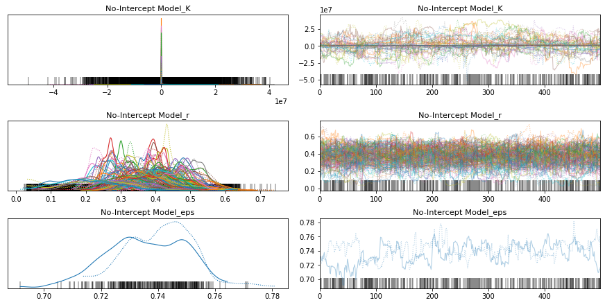
No-Intercept Model
In fact, let me test with a fixed parameter for the intercept. I bet it doesn’t make much difference, so we might as well simplify the model.
no_intercept_model = pm.Model("No-Intercept Model")
with no_intercept_model:
    BoundedNormal = pm.Bound(pm.Normal, lower=0.0)
    t = pm.Data("x_data", sorted_data["days_since_100_cases"])
    confirmed_cases = pm.Data("y_data", sorted_data["cumulative_cases"])

    # Intercept - We fixed this at 100.
    C_0 = 100

    # Growth rate: 0.2 is approx value reported by others
    r = BoundedNormal("r", mu=0.2, sigma=0.1, shape=n_countries)

    # Total number of cases. Depends on the population, more people, more infections.
    proportion_infected = 5e-05 # This value comes from the rough projection that 80000 will be infected in China
    p = sorted_data.popData2018.mean() # Crude. Can have a mean per country. Not sure how to do this
    K = pm.Normal("K", mu=p * proportion_infected, sigma=p*0.1, shape=n_countries)

    # Logistic regression
    growth = logistic(K[idx_country], r[idx_country], t, C_0)

    # Likelihood error
    eps = pm.HalfNormal("eps")

    # Likelihood - Counts here, so poission or negative binomial. Causes issues. Lognormal tends to work better?
    pm.Lognormal("cases", mu=np.log(growth), sigma=eps, observed=confirmed_cases)

pm.model_to_graphviz(no_intercept_model)

with no_intercept_model:
  no_intercept_trace = pm.sample()
pm.traceplot(no_intercept_trace);
pm.forestplot(no_intercept_trace, var_names=[f"{no_intercept_model.name}_r", f"{no_intercept_model.name}_K"]);
Auto-assigning NUTS sampler...
Initializing NUTS using jitter+adapt_diag...
Sequential sampling (2 chains in 1 job)
NUTS: [No-Intercept Model_eps, No-Intercept Model_K, No-Intercept Model_r]
Sampling chain 0, 157 divergences: 100%|██████████| 1000/1000 [05:09<00:00,  3.23it/s]
Sampling chain 1, 166 divergences: 100%|██████████| 1000/1000 [05:12<00:00,  3.20it/s]
There were 158 divergences after tuning. Increase `target_accept` or reparameterize.
The chain reached the maximum tree depth. Increase max_treedepth, increase target_accept or reparameterize.
There were 325 divergences after tuning. Increase `target_accept` or reparameterize.
The chain reached the maximum tree depth. Increase max_treedepth, increase target_accept or reparameterize.
The rhat statistic is larger than 1.4 for some parameters. The sampler did not converge.
The estimated number of effective samples is smaller than 200 for some parameters.
comparison = pm.compare(
    {
      pooled_model.name: pooled_trace,
      total_per_country_model.name: total_per_country_trace,
      growth_per_country_model.name: growth_per_country_trace,
      growth_total_model.name: growth_total_trace,
      everything_model.name: everything_trace,
      no_intercept_model.name: no_intercept_trace
    }, ic='LOO');
print(comparison)
pm.compareplot(comparison);
/usr/local/lib/python3.6/dist-packages/arviz/stats/stats.py:532: UserWarning: Estimated shape parameter of Pareto distribution is greater than 0.7 for one or more samples. You should consider using a more robust model, this is because importance sampling is less likely to work well if the marginal posterior and LOO posterior are very different. This is more likely to happen with a non-robust model and highly influential observations.
  "Estimated shape parameter of Pareto distribution is greater than 0.7 for "
/usr/local/lib/python3.6/dist-packages/arviz/stats/stats.py:532: UserWarning: Estimated shape parameter of Pareto distribution is greater than 0.7 for one or more samples. You should consider using a more robust model, this is because importance sampling is less likely to work well if the marginal posterior and LOO posterior are very different. This is more likely to happen with a non-robust model and highly influential observations.
  "Estimated shape parameter of Pareto distribution is greater than 0.7 for "
/usr/local/lib/python3.6/dist-packages/arviz/stats/stats.py:532: UserWarning: Estimated shape parameter of Pareto distribution is greater than 0.7 for one or more samples. You should consider using a more robust model, this is because importance sampling is less likely to work well if the marginal posterior and LOO posterior are very different. This is more likely to happen with a non-robust model and highly influential observations.
  "Estimated shape parameter of Pareto distribution is greater than 0.7 for "

                   rank      loo    p_loo  ...      dse warning loo_scale
Growth-Total Model    0 -13219.6  98.6516  ...        0    True       log
Total per country     1 -14416.5  52.1214  ...  44.5365   False       log
Growth per country    2 -15052.1  54.3001  ...  66.2718    True       log
Everything Model      3 -16240.9  61.6639  ...  58.6273    True       log
No-Intercept Model    4 -16343.4   43.872  ...  58.1615    True       log
Pooled                5 -16629.8  4.14689  ...   56.487   False       log

[6 rows x 9 columns]
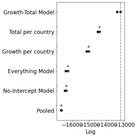
Oh! I was not expecting that. It looks like the model does need some room to manouvre. Ok, so let’s move forward with the growth-total model and see if we can improve upon that with some other distributions.
No Significant Differences
I tried lots of different models and could not find a version that was significantly better. The best improvement was a performance increase, by making the prior for $K$ more general. A broad normal-like distribution helps. A gamma distribution works well, but a broad bounded Normal works just as well.
improved_growth_total_model = pm.Model("Improved GT Model")
with improved_growth_total_model:
    BoundedNormal = pm.Bound(pm.Normal, lower=0.0)
    t = pm.Data("x_data", sorted_data["days_since_100_cases"])
    confirmed_cases = pm.Data("y_data", sorted_data["cumulative_cases"])

    # Intercept - We fixed this at 100.
    C_0 = pm.Normal("C_0", mu=100, sigma=10)

    # Growth rate: 0.2 is approx value reported by others
    r = BoundedNormal("r", mu=0.2, sigma=0.1, shape=n_countries)

    # Total number of cases. Depends on the population, more people, more infections.
    K = pm.Gamma("K", mu=30000, sigma=30000, shape=n_countries)

    # Logistic regression
    growth = logistic(K[idx_country], r[idx_country], t, C_0)

    # Likelihood error
    eps = pm.HalfNormal("eps")

    # Likelihood - Counts here, so poission or negative binomial. Causes issues. Lognormal tends to work better?
    pm.Lognormal("cases", mu=np.log(growth), sigma=eps, observed=confirmed_cases)

pm.model_to_graphviz(improved_growth_total_model)

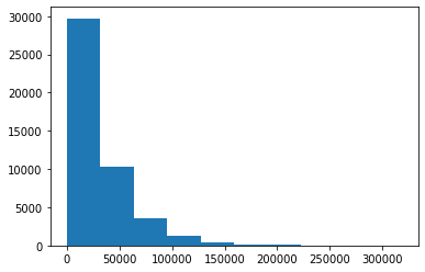
# Check what the negative binomial / K prior looks like
with improved_growth_total_model:
  prior = pm.sample_prior_predictive()
# prior.keys()
plt.hist(prior['Improved GT Model_K'].flatten());
plt.show()
for RV in improved_growth_total_model.basic_RVs:
    print(RV.name, RV.logp(improved_growth_total_model.test_point))
Improved GT Model_C_0 -3.2215236261987186
Improved GT Model_r_lowerbound__ -2786.0881630591693
Improved GT Model_K_log__ -91.0
Improved GT Model_eps_log__ -0.7698925914732455
Improved GT Model_cases -20863.226039690697
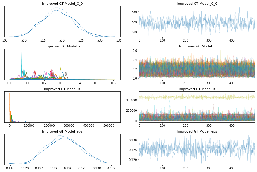
with improved_growth_total_model:
improved_growth_total_trace = pm.sample()
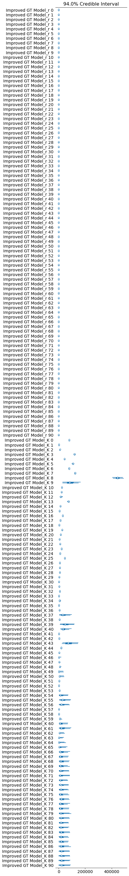
pm.traceplot(improved_growth_total_trace);
pm.forestplot(improved_growth_total_trace, var_names=[f"{improved_growth_total_model.name}_r", f"{improved_growth_total_model.name}_K"]);
Auto-assigning NUTS sampler...
Initializing NUTS using jitter+adapt_diag...
Sequential sampling (2 chains in 1 job)
NUTS: [Improved GT Model_eps, Improved GT Model_K, Improved GT Model_r, Improved GT Model_C_0]
Sampling chain 0, 0 divergences: 100%|██████████| 1000/1000 [01:05<00:00, 15.22it/s]
Sampling chain 1, 0 divergences: 100%|██████████| 1000/1000 [00:53<00:00, 18.70it/s]
The estimated number of effective samples is smaller than 200 for some parameters.
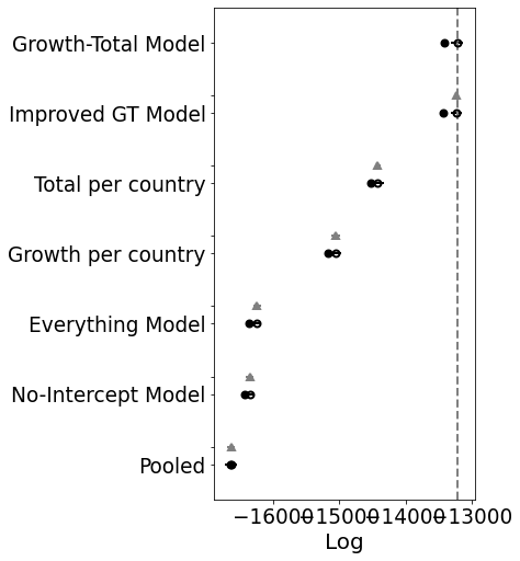
comparison = pm.compare(
    {
      pooled_model.name: pooled_trace,
      total_per_country_model.name: total_per_country_trace,
      growth_per_country_model.name: growth_per_country_trace,
      growth_total_model.name: growth_total_trace,
      everything_model.name: everything_trace,
      no_intercept_model.name: no_intercept_trace,
      improved_growth_total_model.name: improved_growth_total_trace,
    }, ic='LOO');
print(comparison)
pm.compareplot(comparison);
/usr/local/lib/python3.6/dist-packages/arviz/stats/stats.py:532: UserWarning: Estimated shape parameter of Pareto distribution is greater than 0.7 for one or more samples. You should consider using a more robust model, this is because importance sampling is less likely to work well if the marginal posterior and LOO posterior are very different. This is more likely to happen with a non-robust model and highly influential observations.
  "Estimated shape parameter of Pareto distribution is greater than 0.7 for "
/usr/local/lib/python3.6/dist-packages/arviz/stats/stats.py:532: UserWarning: Estimated shape parameter of Pareto distribution is greater than 0.7 for one or more samples. You should consider using a more robust model, this is because importance sampling is less likely to work well if the marginal posterior and LOO posterior are very different. This is more likely to happen with a non-robust model and highly influential observations.
  "Estimated shape parameter of Pareto distribution is greater than 0.7 for "
/usr/local/lib/python3.6/dist-packages/arviz/stats/stats.py:532: UserWarning: Estimated shape parameter of Pareto distribution is greater than 0.7 for one or more samples. You should consider using a more robust model, this is because importance sampling is less likely to work well if the marginal posterior and LOO posterior are very different. This is more likely to happen with a non-robust model and highly influential observations.
  "Estimated shape parameter of Pareto distribution is greater than 0.7 for "
/usr/local/lib/python3.6/dist-packages/arviz/stats/stats.py:532: UserWarning: Estimated shape parameter of Pareto distribution is greater than 0.7 for one or more samples. You should consider using a more robust model, this is because importance sampling is less likely to work well if the marginal posterior and LOO posterior are very different. This is more likely to happen with a non-robust model and highly influential observations.
  "Estimated shape parameter of Pareto distribution is greater than 0.7 for "

                   rank      loo    p_loo  ...      dse warning loo_scale
Growth-Total Model    0 -13219.6  98.6516  ...        0    True       log
Improved GT Model     1 -13232.9  101.091  ...  2.77116    True       log
Total per country     2 -14416.5  52.1214  ...  44.5365   False       log
Growth per country    3 -15052.1  54.3001  ...  66.2718    True       log
Everything Model      4 -16240.9  61.6639  ...  58.6273    True       log
No-Intercept Model    5 -16343.4   43.872  ...  58.1615    True       log
Pooled                6 -16629.8  4.14689  ...   56.487   False       log

[7 rows x 9 columns]
Hierarchical Bayesian Model
Ok you’re finally there. Congratulations if you’ve stuck with me this far!
Previously we were generating parameter estimates for each country individually. This probably doesn’t make sense, since this is the same virus after all. They are all linked at some level.
At first I just tried to tie the rate of infection (the $r$ parameter), but I thought I might as well tie the K parameter too. On some level, there is going to be a similar level of infected population. But I can imagine a more complex model here taking the population and distribution of people into account.
In summary then, below is a model that assumes that the prior $r$ and $K$ estimates for a country have their means and standard deviations sampled from a high-level abstraction. The global distribution of $r$ and $K$.
This should help countries that have little data to produce a better initial estimate for their $r$ and $K$. Their estimate should be constrained to lie somewhere within the global distribution.
hierarchical_model = pm.Model("Hierarchical Model")
with hierarchical_model:
    BoundedNormal = pm.Bound(pm.Normal, lower=0.0)
    t = pm.Data("x_data", sorted_data["days_since_100_cases"])
    confirmed_cases = pm.Data("y_data", sorted_data["cumulative_cases"])

    # Intercept - We fixed this at 100.
    C_0 = pm.Normal("C_0", mu=100, sigma=10)

    # Growth rate: 0.2 is approx value reported by others
    r_mu = pm.Normal("r_mu", mu=0.2, sigma=0.1)
    r_sigma = pm.HalfNormal("r_sigma", 0.5)
    r = BoundedNormal("r", mu=r_mu, sigma=r_sigma, shape=n_countries)

    # Total number of cases. Depends on the population, more people, more infections.
    K_mu = pm.Normal("K_mu", mu=30000, sigma=30000)
    K_sigma = pm.HalfNormal("K_sigma", 1000)
    K = pm.Gamma("K", mu=K_mu, sigma=K_sigma, shape=n_countries)

    # Logistic regression
    growth = logistic(K[idx_country], r[idx_country], t, C_0)

    # Likelihood error
    eps = pm.HalfNormal("eps")

    # Likelihood - Counts here, so poission or negative binomial. Causes issues. Lognormal tends to work better?
    pm.Lognormal("cases", mu=np.log(growth), sigma=eps, observed=confirmed_cases)

pm.model_to_graphviz(hierarchical_model)

for RV in hierarchical_model.basic_RVs:
    print(RV.name, RV.logp(hierarchical_model.test_point))
Hierarchical Model_C_0 -3.2215236261987186
Hierarchical Model_r_mu 1.3836465597893728
Hierarchical Model_r_sigma_log__ -0.7698925914732455
Hierarchical Model_r_lowerbound__ -182.96635614506937
Hierarchical Model_K_mu -11.227891193848965
Hierarchical Model_K_sigma_log__ -0.7698925914732451
Hierarchical Model_K_log__ 246.42720418948204
Hierarchical Model_eps_log__ -0.7698925914732455
Hierarchical Model_cases -20863.226039690697
with hierarchical_model:
hierarchical_trace = pm.sample()
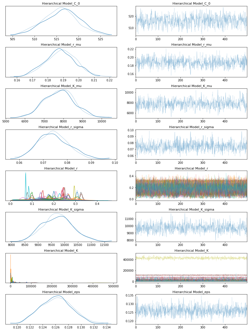
pm.traceplot(hierarchical_trace);
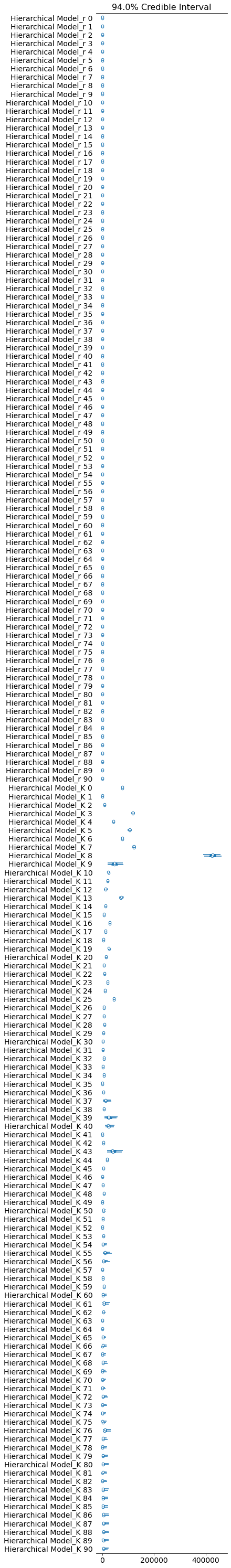
pm.forestplot(hierarchical_trace, var_names=[f"{hierarchical_model.name}_r", f"{hierarchical_model.name}_K"]);
Auto-assigning NUTS sampler...
Initializing NUTS using jitter+adapt_diag...
Sequential sampling (2 chains in 1 job)
NUTS: [Hierarchical Model_eps, Hierarchical Model_K, Hierarchical Model_K_sigma, Hierarchical Model_K_mu, Hierarchical Model_r, Hierarchical Model_r_sigma, Hierarchical Model_r_mu, Hierarchical Model_C_0]
Sampling chain 0, 0 divergences: 100%|██████████| 1000/1000 [01:03<00:00, 15.87it/s]
Sampling chain 1, 0 divergences: 100%|██████████| 1000/1000 [00:49<00:00, 20.27it/s]
The rhat statistic is larger than 1.05 for some parameters. This indicates slight problems during sampling.
The estimated number of effective samples is smaller than 200 for some parameters.
comparison = pm.compare(
    {
      pooled_model.name: pooled_trace,
      total_per_country_model.name: total_per_country_trace,
      growth_per_country_model.name: growth_per_country_trace,
      growth_total_model.name: growth_total_trace,
      everything_model.name: everything_trace,
      no_intercept_model.name: no_intercept_trace,
      improved_growth_total_model.name: improved_growth_total_trace,
      hierarchical_model.name: hierarchical_trace,
    }, ic='LOO');
print(comparison)
pm.compareplot(comparison);
/usr/local/lib/python3.6/dist-packages/arviz/stats/stats.py:532: UserWarning: Estimated shape parameter of Pareto distribution is greater than 0.7 for one or more samples. You should consider using a more robust model, this is because importance sampling is less likely to work well if the marginal posterior and LOO posterior are very different. This is more likely to happen with a non-robust model and highly influential observations.
  "Estimated shape parameter of Pareto distribution is greater than 0.7 for "
/usr/local/lib/python3.6/dist-packages/arviz/stats/stats.py:532: UserWarning: Estimated shape parameter of Pareto distribution is greater than 0.7 for one or more samples. You should consider using a more robust model, this is because importance sampling is less likely to work well if the marginal posterior and LOO posterior are very different. This is more likely to happen with a non-robust model and highly influential observations.
  "Estimated shape parameter of Pareto distribution is greater than 0.7 for "
/usr/local/lib/python3.6/dist-packages/arviz/stats/stats.py:532: UserWarning: Estimated shape parameter of Pareto distribution is greater than 0.7 for one or more samples. You should consider using a more robust model, this is because importance sampling is less likely to work well if the marginal posterior and LOO posterior are very different. This is more likely to happen with a non-robust model and highly influential observations.
  "Estimated shape parameter of Pareto distribution is greater than 0.7 for "
/usr/local/lib/python3.6/dist-packages/arviz/stats/stats.py:532: UserWarning: Estimated shape parameter of Pareto distribution is greater than 0.7 for one or more samples. You should consider using a more robust model, this is because importance sampling is less likely to work well if the marginal posterior and LOO posterior are very different. This is more likely to happen with a non-robust model and highly influential observations.
  "Estimated shape parameter of Pareto distribution is greater than 0.7 for "
/usr/local/lib/python3.6/dist-packages/arviz/stats/stats.py:532: UserWarning: Estimated shape parameter of Pareto distribution is greater than 0.7 for one or more samples. You should consider using a more robust model, this is because importance sampling is less likely to work well if the marginal posterior and LOO posterior are very different. This is more likely to happen with a non-robust model and highly influential observations.
  "Estimated shape parameter of Pareto distribution is greater than 0.7 for "

                   rank      loo    p_loo  ...      dse warning loo_scale
Growth-Total Model    0 -13219.6  98.6516  ...        0    True       log
Improved GT Model     1 -13232.9  101.091  ...  2.77116    True       log
Hierarchical Model    2 -13243.7  97.9735  ...  4.41949    True       log
Total per country     3 -14416.5  52.1214  ...  44.5365   False       log
Growth per country    4 -15052.1  54.3001  ...  66.2718    True       log
Everything Model      5 -16240.9  61.6639  ...  58.6273    True       log
No-Intercept Model    6 -16343.4   43.872  ...  58.1615    True       log
Pooled                7 -16629.8  4.14689  ...   56.487   False       log

[8 rows x 9 columns]
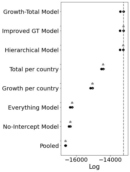
Ok, so the score doesn’t look much better. BUT. And that’s a big but. Look at the posteriors for the latter K’s. Those are the countries that don’t have many samples yet.
Plots Using the Hierarchical model vs. Original
Previously the estimates were wildly inaccurate because we were effectively trying to train a model on a handful of observations. But now, we’re using pooled knowledge to predict the new values.
Let me plot the predictions from the GT model against the hierarchical model for comparison.
Apologies for the code duplication.
country = "Tunisia"
x = range(60)
y = np.zeros(len(x))
x_obs = sorted_data[sorted_data.country == country]["days_since_100_cases"]
y_obs = sorted_data[sorted_data.country == country]["cumulative_cases"]
current_country = np.argmax(countries == country)
test_model = pm.Model("Hierarchical Model")
with test_model:
    BoundedNormal = pm.Bound(pm.Normal, lower=0.0)
    t = pm.Data("x_data", x)
    confirmed_cases = pm.Data("y_data", y)

    # Intercept - We fixed this at 100.
    C_0 = pm.Normal("C_0", mu=100, sigma=10)

    # Growth rate: 0.2 is approx value reported by others
    r_mu = pm.Normal("r_mu", mu=0.2, sigma=0.1)
    r_sigma = pm.HalfNormal("r_sigma", 0.5)
    r = BoundedNormal("r", mu=r_mu, sigma=r_sigma, shape=n_countries)

    # Total number of cases. Depends on the population, more people, more infections.
    K_mu = pm.Normal("K_mu", mu=30000, sigma=30000)
    K_sigma = pm.HalfNormal("K_sigma", 1000)
    K = pm.Gamma("K", mu=K_mu, sigma=K_sigma, shape=n_countries)

    # Logistic regression
    growth = logistic(K[current_country], r[current_country], t, C_0)

    # Likelihood error
    eps = pm.HalfNormal("eps")

    # Likelihood - Counts here, so poission or negative binomial. Causes issues. Lognormal tends to work better?
    pm.Lognormal("cases", mu=np.log(growth), sigma=eps, observed=confirmed_cases)

pm.model_to_graphviz(test_model)

# New model with holdout data
with test_model:
  ppc_hierarchical = pm.sample_posterior_predictive(hierarchical_trace)
100%|██████████| 1000/1000 [00:11<00:00, 84.37it/s]
test_model_poor = pm.Model("Growth-Total Model")
with test_model_poor:
    BoundedNormal = pm.Bound(pm.Normal, lower=0.0)
    t = pm.Data("x_data", x)
    confirmed_cases = pm.Data("y_data", y)

    # Intercept - We fixed this at 100.
    C_0 = pm.Normal("C_0", mu=100, sigma=10)

    # Growth rate: 0.2 is approx value reported by others
    r = BoundedNormal("r", mu=0.2, sigma=0.1, shape=n_countries)

    # Total number of cases. Depends on the population, more people, more infections.
    proportion_infected = 5e-05 # This value comes from the rough projection that 80000 will be infected in China
    p = sorted_data.popData2018.mean() # Crude. Can have a mean per country. Not sure how to do this
    K = pm.Normal("K", mu=p * proportion_infected, sigma=p*0.1, shape=n_countries)

    # Logistic regression
    growth = logistic(K[current_country], r[current_country], t, C_0)

    # Likelihood error
    eps = pm.HalfNormal("eps")

    # Likelihood - Counts here, so poission or negative binomial. Causes issues. Lognormal tends to work better?
    pm.Lognormal("cases", mu=np.log(growth), sigma=eps, observed=confirmed_cases)

pm.model_to_graphviz(test_model_poor)

# New model with holdout data
with test_model_poor:
  ppc_gt = pm.sample_posterior_predictive(growth_total_trace)
100%|██████████| 1000/1000 [00:11<00:00, 84.95it/s]
  fig, ax = plt.subplots(nrows=1, ncols=2, figsize=(15, 7))
  ax[0].plot(x, ppc_gt["Growth-Total Model_cases"].T, ".k", alpha=0.05)
  ax[0].plot(x_obs, y_obs, color="r")
  ax[0].plot(x, np.mean(ppc_gt["Growth-Total Model_cases"], axis=0), "b", alpha=0.5)
  ax[0].set_yscale("log")
  ax[0].set(xlabel="Date", ylabel="Confirmed Cases", title=f"{country} - Standard GT model");
  ax[1].plot(x, ppc_hierarchical["Hierarchical Model_cases"].T, ".k", alpha=0.05)
  ax[1].plot(x_obs, y_obs, color="r")
  ax[1].plot(x, np.mean(ppc_hierarchical["Hierarchical Model_cases"], axis=0), "b", alpha=0.5)
  ax[1].set_yscale("log")
  ax[1].set(xlabel="Date", ylabel="Confirmed Cases", title=f"{country} - Hierarchical GT model");
  plt.show()
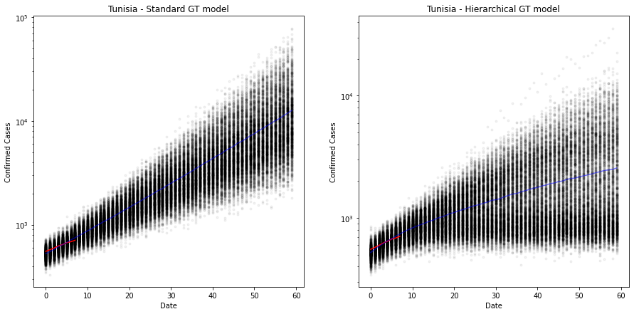
The plot above shows the predicted number of cases over 60 days from the first 100 cases. The old model is still very exponential and has quite a narrow error band, suggesting that there is less error in the estimate than there really is. Look at the red line, it is clearly projecting downward.
On the right we have the hierarchical model. The estimate is now much more conservative, but crucially, the error bands are much wider, suggesting a lack of confidence (as it should, given that there are only 7 observations here).
It suggests that Tunisia will have somewhere around 1000 cases around day 20 (approximately 27th April 2020). But the credible interval (95%) around that is 500-2000. Very wide. Especially given that they have already passed the 500 mark! :-)
Out of interest, the total number of infections for Tunisia, K, is around 4400 at the moment (14/04/20).
Ideally we want to improve these confidence bounds. But I’ll leave that for another day.
hierarchical_trace["Hierarchical Model_K"][:,current_country].mean()
4394.678726322066