COVID-19 Exponential Bayesian Model
by Dr. Phil Winder , CEO
The purposes of this notebook is to provide initial experience with the pymc3 library for the purpose of modeling and forecasting COVID-19 virus summary statistics. This model is very simple, and therefore not very accurate, but serves as a good introduction to the topic.
This was heavily inspired by Thomas Wiecki from a video about this very topic.
Further analysis, questions and models to follow.
Not doing
- Iterate over countries
- Start work on more complex models (e.g. SIR/etc., heirarchical)
- Investigate and justify different priors
- Implement back testing
- Implement cross-validation with other countries
- Consider segmenting countries (see analysis notebook)
Initialisation
Initial installation and importing.
!pip install arviz pymc3==3.8
import numpy as np
import pymc3 as pm
import pandas as pd
import matplotlib.pyplot as plt
Load the Data
This is using global ECDC data. Note that the dates are in European format. I rename columns for sanity and remove unnecessary columns.
df = pd.read_csv("https://opendata.ecdc.europa.eu/covid19/casedistribution/csv/", parse_dates=["dateRep"], infer_datetime_format=True, dayfirst=True)
df = df.rename(columns={'dateRep': 'date', 'countriesAndTerritories': 'country'}) # Sane column names
df = df.drop(["day", "month", "year", "geoId"], axis=1) # Not required
Filter for a single country, just to get used to the data. In more sophisticated versions we can look at all countries.
# Filter for country (probably want separate models per country, even maybe per region)
country = df[df["country"] == "United_Kingdom"].sort_values(by="date")
# Cumulative sum of data
country_cumsum = country[["cases", "deaths"]].cumsum().set_index(country["date"])
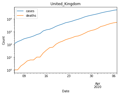
# Filter out data with less than 100 cases
country_cumsum = country_cumsum[country_cumsum["cases"] >= 100]
country_cumsum.plot(logy=True)
plt.gca().set(xlabel="Date", ylabel="Count", title="United_Kingdom")
plt.show()
The First Model
This is where we specify our model, a very simple exponential model to begin with.
One of the major benefits of doing a Bayesian analysis is that we can include prior beliefs, to help fit our model. The priors come in the form of an expected distribution. I chose normal distributions for simplicity. {More analysis required here}.
The first prior is to provide an intercept. We need that to account for the offset at the beginning of the data (I restricted the data to wait for 100 confirmed cases). A normal distribution for this.
Next, we add a growth rate. The value of 0.2 is appropriate prior based upon previous research (see Appendix 1).
Then we define the exponential model and fit the parameters.
country = "United_Kingdom"
days_since_100 = range(len(country_cumsum))

# Create PyMC3 context manager
with pm.Model() as model:
  t = pm.Data(country + "x_data", days_since_100)
  confirmed_cases = pm.Data(country + "y_data", country_cumsum["cases"].astype('float64').values)

  # Intercept - We fixed this at 100.
  a = pm.Normal("a", mu=100, sigma=10)

  # Slope - Growth rate: 0.2 is approx value reported by others
  b = pm.Normal("b", mu=0.2, sigma=0.5)

  # Exponential regression
  growth = a * (1 + b) ** t

  # Likelihood error
  eps = pm.HalfNormal("eps")

  # Likelihood - Counts here, so poission or negative binomial. Causes issues. Lognormal tends to work better?
  pm.Lognormal(country, mu=np.log(growth), sigma=eps, observed=confirmed_cases)

  trace = pm.sample()
  post_Pred = pm.sample_posterior_predictive(trace)
Auto-assigning NUTS sampler...
Initializing NUTS using jitter+adapt_diag...
Sequential sampling (2 chains in 1 job)
NUTS: [eps, b, a]
Sampling chain 0, 0 divergences: 100%|██████████| 1000/1000 [00:03<00:00, 277.16it/s]
Sampling chain 1, 0 divergences: 100%|██████████| 1000/1000 [00:02<00:00, 413.72it/s]
The acceptance probability does not match the target. It is 0.8999537134484051, but should be close to 0.8. Try to increase the number of tuning steps.
100%|██████████| 1000/1000 [00:10<00:00, 94.66it/s]
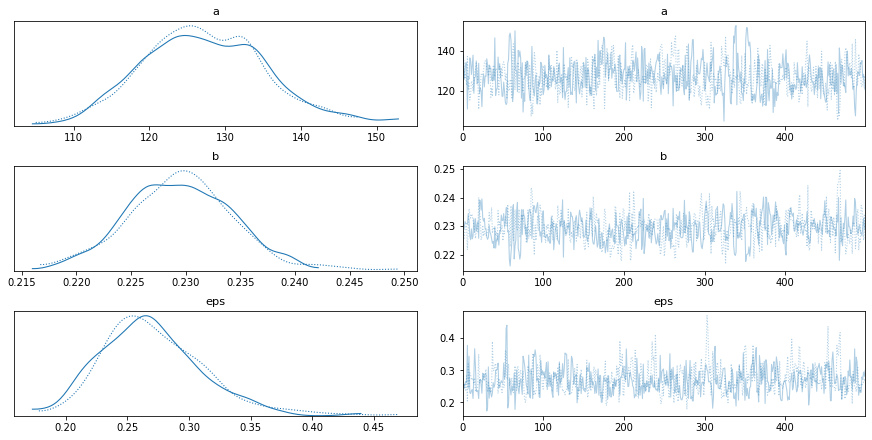
Now that the model is trained we can take a look at the fitted values over multiple runs.
Traceplots show model parameters over time. Each line represents a sampling chain in the MCMC sampling. The distributions should be similar and the raw traces should be stationary and converge to similar values when repeated.
pm.traceplot(trace)
plt.show()
Result
Here is the final result of the model. In the table below, mean represents the predicted values for the parameters of the model, sd is the estimated standard deviation, hpd_x is the upper and lower bound of the interval where a parameter falls with a certain probability, mcse is the monte carlo standard error (a measure of similarity between posterior estimates) and should be low. ess is the effective sample size (a measure of autocorrelation along the trace) and should be high and r_hat is an estimate of how converged chains have become (chains that end in different positions will have a near zero value) and should be near 1.
pm.summary(trace).round(2)
| mean | sd | hpd_3% | hpd_97% | mcse_mean | mcse_sd | ess_mean | ess_sd | ess_bulk | ess_tail | r_hat | |
|---|---|---|---|---|---|---|---|---|---|---|---|
| a | 127.18 | 8.12 | 112.44 | 142.84 | 0.38 | 0.27 | 449.0 | 442.0 | 459.0 | 472.0 | 1.0 |
| b | 0.23 | 0.00 | 0.22 | 0.24 | 0.00 | 0.00 | 472.0 | 472.0 | 473.0 | 544.0 | 1.0 |
| eps | 0.27 | 0.04 | 0.20 | 0.35 | 0.00 | 0.00 | 496.0 | 485.0 | 518.0 | 553.0 | 1.0 |
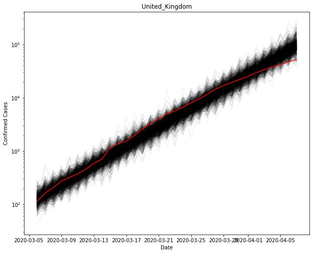
Using the values for the parameters, you can sample new observations and see how they compare to the original.
fig, ax = plt.subplots(figsize=(10, 8))
ax.plot(country_cumsum.index, post_Pred[country].T, color="k", alpha=0.05)
ax.plot(country_cumsum.index, country_cumsum["cases"].astype('float64').values, color="r")
ax.set_yscale("log")
ax.set(xlabel="Date", ylabel="Confirmed Cases", title=country)
plt.show()
Appendix 1: Exponential growth rates
There are a variety of fitted growth rates appearing in the literature. Could spend all day reading about it. It looks like a value of 0.2 is appropriate for larger countries.
- India (0.18-0.19), Ganesh Kumar et al., http://arxiv.org/abs/2003.12017
- China (0.24), Wu et al., https://arxiv.org/pdf/2003.05681.pdf
- China (0.22), Batista, https://www.medrxiv.org/content/10.1101/2020.03.11.20024901v2.full.pdf