403: Linear Classification

Classification via a model

Decision trees created a one-dimensional decision boundary
We could easily imagine using a linear model to define a decision boundary

???

Previously we used fixed decision boundaries to segment the data based upon how informative the segmentation would be.

The decision boundary represents a one-dimensional rule that separates the data. We could easily increase the number or complexity of the parameters used to define the boundary.

Leaving the decision boundary parameters unspecified, we can allow the parameters to be defined by some theoretical model or by some regression-like process.

Modelling

In the extreme, we can use any arbitrary function to define a decision boundary.

But some interesting questions arise:

What is the optimal location for the boundary?
What do we mean by optimal?
How can we justify a boundary, in business terms?

???

Many types of problems can be defined in this way and there are a range of linear and nonlinear methods that are able to define the decision boundary.

Classification via mathematical functions

Consider the image below. The data has two features.

If we used one-dimensional rules, like in a decision tree, we would end up with a decision boundary looking like this:

Linear function

Instead, we could create a decision boundary that is a mathematical function. Like this:

This type of decision boundary is called a linear classifier because the hyperplane is a weighted combination of linear features. E.g. $y = mx + c$

More generally, a linear function is defined as:

\begin{align} f(\mathbf{x}) & = w_0 + w_1x_1 + w_2x_2 + \dots \\ & = \mathbf{w} ^T \cdot \mathbf{x} \end{align}

This is the same as linear regression!

The goal, however is different. The goal is to alter the parameters $\mathbf{w}$ so that it correctly classifies all classes in the data $\mathbf{x}$.

But this begs the question, what is the best location for the decision boundary?

We could place the decision boundary in any number of locations:

Which is best? This leads us to one of the most important questions in data science, one that is often overlooked, but is the key to advanced applications…

Loss Function

What is the goal or objective when choosing the parameters?

The general procedure is to define an objective, then optimise the parameters to fulfil that objective (as best as it can).

Note: The premise is the same as a cost function, but now we’re talking about categorical classes.

???

For example, we could choose the objective function to optimally separate classes or we could be interested in being as far away as one class as possible (to avoid false positives, for example).

The choice of loss function is often quite hard to define and a range of “standard” objective functions have emerged:

Linear
Support Vector Machines
Logistic

These three are the workhorses of data science and differ only in their objective.

class: center, middle

Example: Petal/Sepal

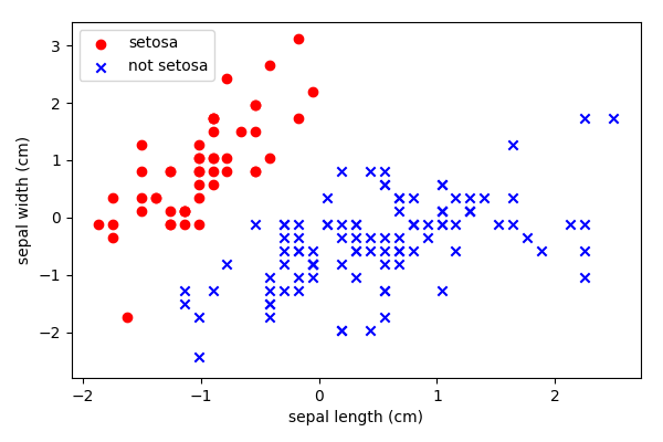
The Iris dataset is one of a number of “standard” data science datasets.

???

It is a dataset that measures different parts of an iris flower and is labeled by the species.

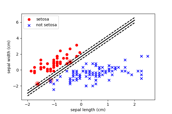
Two of the features are plotted below for two of the species.

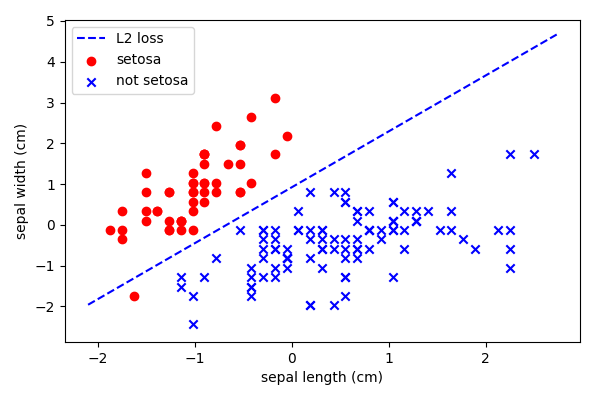
Linear Classification

This measures the squared error between the distance from the boundary to a misclassification.

???

This attempts to fit a line that best reduces the squared error of two or more classes. For these examples we will use stochastic gradient descent.

We can see that there are some issues with this classification.

Skewed due to larger numbers of one class
Sensitive to outliers (assumes gaussian distribution)
Does the chosen objective match to the business requirements? E.g. are those misclassifications costly?

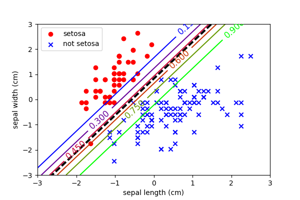
Logistic regression

Logistic regression is often used because it also estimates class probabilities.

Logistic regression fits a binomial distribution between two classes. A probability of 0.5 is used as the decision boundary.

???

Logistic regression (a.k.a. logit regression) is commonly used to estimate the probability that a new observation belongs to a class of interest. For example, if the goal is to reduce the amount of money lost to fraud, then we not only need to know the occurance of fraud, but also the probability of it occurring.

Logistic regression is a linear model that instead of outputting expected value directly, it outputs the logistic of this result:

$$ \hat{p} = h_w(\mathbf{x}) = \sigma(\mathbf{w}^T \cdot \mathbf{x}) $$

The logistic, (a.k.a. logit) is a sigmoid function that outputs a number between 0 and 1.

$$ \sigma(t) = \frac{1}{1 + \exp(-t)} $$

Once the model has estimated the probability of the class $\hat{p}$ it can threshold at a value of 0.5 to perform classification.

Training

Assuming binary classification, we need a cost function that produces a small value when the regression correctly predicts a class and a large value when it gets it wrong. Commonly, this is used:

$$ c(w) = \begin{cases} -\log{\left(\hat{p}\right)}, & \text{if y = 1} \\ \log{\left(1 - \hat{p}\right)}, & \text{if y = 0} \\ \end{cases} $$

The cost function is then the average log error over the entire dataset. This is a common loss function and so has a name, the log loss:

$$ J(w) = \frac{1}{m} \sum_{i=1}^{m}{ \left(y^{(i)} \log{ \left( \hat{p}^{(i)} \right)} + (1 - y^{(i)}) \log{\left(1 - \hat{p}\right)} \right)} $$

Unfortunately there is no closed solution so we must use an optimisation algorithm to find the solution. Thankfully though it is convex so the solution guaranteed to find the global minimum. It also looks very similar to the MSE’s partial derivative.

$$ \frac{\partial}{\partial \mathbf{w}_j} J(\mathbf{w}) = \frac{2}{m} \sum_{i=1}^{m} \left( \sigma \left(\mathbf{w}^T \cdot \mathbf{x}^{(i)} - \mathbf{y}^{(i)} \right)\right) \mathbf{x}^{(i)}_j $$

This is the result of logistic regression (a.k.a. fitting a binomial distribution).

Support vector machines

SVMs have an annoyingly vague name, but their performance is impressive.

They have one goal:

Maximise the boundary between classes

It tries to separate the classes by the largest possible margin:

???

First, it classifies using a hard margin. I.e. anything above the threshold has no penalty and anything below it has increasing penalty.

The loss function that achieves this is a loss of 0 at correct classifications and an increasing loss at at incorrect classifications. This is very similar to a magnitude loss (L1) except there is a classification discontinuity at 0.

The issue with this is that because it’s discontinuous, it isn’t differentiable. Which means we can’t use any of the gradient descent methods. Instead, it resorts to a pretty complex form of linear algebra called Quadratic Programming.

It allows some points into the margin by using a Hinge loss (i.e. it continues to penalise elements within the margin)

We can see that it has positioned the threshold to produce correct classifications, but has allowed observations to enter the margin.

Note, however, that because of the outlier in the bottom left, it is still skewing the decision boundary to be slightly higher than (in my opinion) it should. And this is why many people prefer logistic regression…

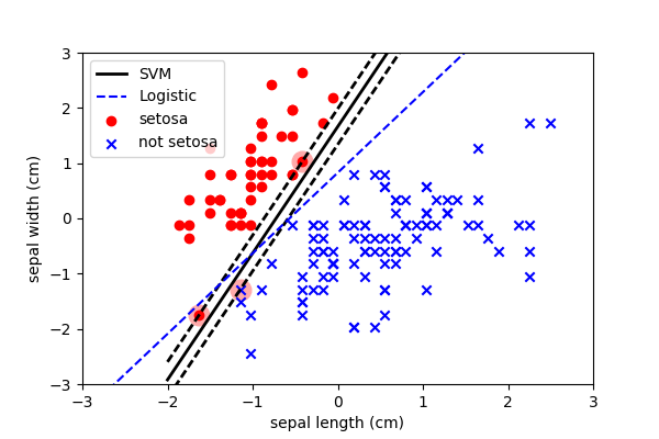
And this is ultimately because of the cost function…

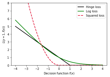
Remember: Loss Function

Remember that the only difference between these three algorithms is the function used to calculate the loss.