402: Optimisation and Gradient Descent

Optimisation

When discussing regression we found that these have closed solutions. I.e. solutions that can be solved directly. For many other algorithms there is no closed solution available.

In these cases we need to use an optimisation algorithm. The goals of these algorithms is to iteratively step towards the correct result.

Gradient descent

Given a cost function, the gradient decent algorithm calculates the gradient of the last step and move in the direction of that gradient.

Important: Step size, stopping.

???

Once the gradient approaches zero, then we stop. The step size is an important parameter. Too low, it will take too long. Too high and it will overshoot the minima.

Issues with gradient descent

The gradient of linear regression produces a single, closed solution.

But generally, most data science algorithms have many minima (e.g. a quadratic has two solutions).

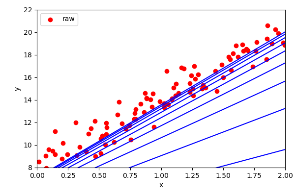
Implementation of gradient descent

1. Calculate the partial derivative of the cost function
2. Iteratively update the values of the weights to traverse down the slope

???

We need to calculate the gradient of the cost function. I.e. we need to calculate the difference between a step of a single parameter. This is known as the partial derivative:

$$ \frac{\partial}{\partial \mathbf{w}_j} MSE(\mathbf{w}) = \frac{2}{m} \sum_{i=1}^{m} \left(\mathbf{w}^T \cdot \mathbf{x}^{(i)} - \mathbf{y}^{(i)} \right) \mathbf{x}^{(i)}_j $$

Instead of calculating the derivatives for the parameters individually, we can compute them in one fell swoop with the gradient vector:

$$ \nabla_{\mathbf{w}} MSE(\mathbf{w}) = \frac{2}{m}\mathbf{x}^T \cdot (\mathbf{x} \cdot \mathbf{w} - \mathbf{y}) $$

Note how this uses every element in the dataset.

Implementation:

???

eta = 0.1 # learning rate
n_iterations = 1000 # number of iterations
m=100 # number of observations

w = np.random.randn(2,1) # random initialization of parameters
for iteration in range(n_iterations):
    gradients = 2/m * X_b.T.dot(X_b.dot(w) - y)
    w = w - eta * gradients

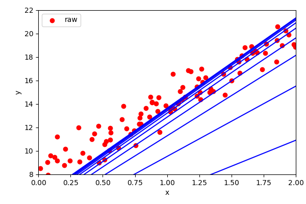
Stochastic Gradient Descent

Standard gradient descent:

• Uses all data for each update (RAM limited)
• Gets stuck on plateaus and in local minima

Stochastic gradient descent is a fancy name for:

• Updating the weights in smaller batches (minibatches), often one observation at a time

Need to randomise data

???

So there are several issues with standard gradient descent:

• Uses all the data at once, probably won’t fit in RAM
• Gets stuck in local minima and plateaus

One thing we can do is run through the data in a loop, rather than running it as one big matrix equation. Or subsets of the data to gain some of the optimisations made by matrix math libraries (this is called minibatch gradient descent).

But the result would be that we would be fitting to an ordered version of the data. So each time we need to either randomise the data, or simply pick a observation at random.

Despite this, it is actually remarkably useful, because the “jitter” causes it to jump out of local minima and plateaus. But this means it never really settles at a minima. We can control this by reducing the learning rate as we go.

Foreach iteration
    Foreach observation
        pick a random index
        calculate gradient for single observation
        reduce the step size slightly
        update w

Implementation

n_iterations = 10
m=100 # number of observations
t0, t1 = 5, 50 # learning schedule hyperparameters

def learning_schedule(t):
    return t0/(t+t1)

w = np.random.randn(2,1) # random initialization
for iteration in range(n_iterations):
    for i in range(m):
        random_index = np.random.randint(m)
        xi = X_b[random_index:random_index+1]
        yi = y[random_index:random_index+1]
        gradients = 2 * xi.T.dot(xi.dot(w) - yi)
        eta = learning_schedule(epoch * m + i)
        w = w - eta * gradients

This type of learning schedule is known as simulated annealing (from metalurgy, where annealing is the process of metal slowly cooling).